Data Assimilation demo in the Lorenz 96 (L96) two time-scale model#
What is DA? Why do we do it?#
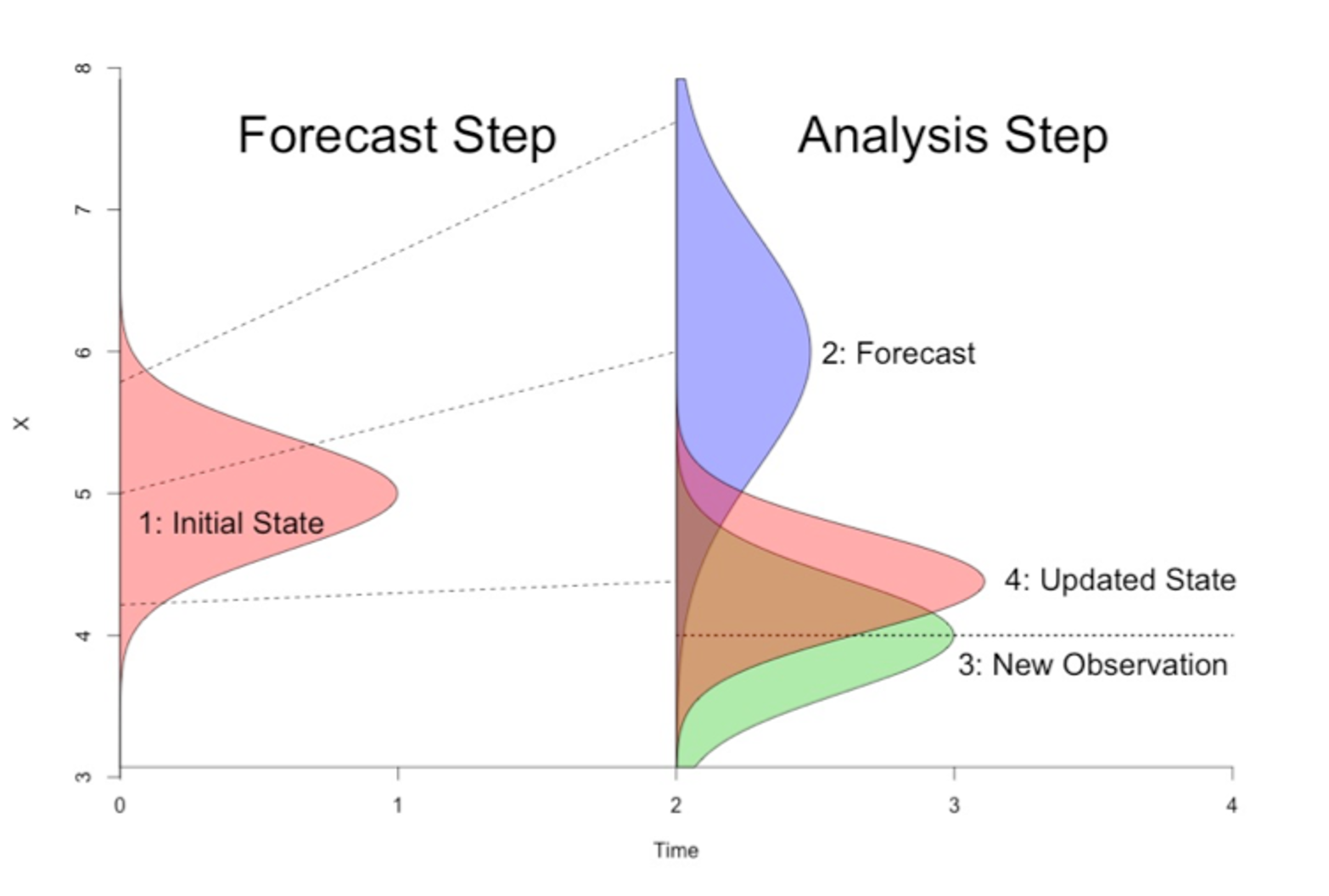
Data assimilation is an approach for combining data (e.g. observations) with prior knowledge (e.g. from a physical model) to obtain an estimate of the true state of a system. We use data assimilation to generate accurate initial conditions for weather and climate predictions, and to produce reanalysis products (state estimates) of the atmosphere-ocean-sea ice-land system.
Conceptually, data assimilation follows the Bayes’ Rule:
where \(X\) is the state of the dynamic system, \(P(X|Obs)\) is the posterior distribution, or the analysis in DA terms, and \(P(X)\) is the prior distribution, or the forecast in DA terms. \(P(Obs|X)\) is the observation distribution given the prior. Simply speaking, we want to know the best estimate of the current state \(X\) of the system given the available observations. Below is a simple schematic representation of one DA step.
Design of the data assimilation experiments in L96#
We use the 2-scale Lorenz-96 model as our truth, or our representation of the “real world”. We then use the 1-scale L96 model as our DA model, or our representation of the “GCM”. Detailed description of this setup can be find here (https://m2lines.github.io/L96_demo/notebooks/gcm-analogue.html). This is what we call an idealized biased-model framework in DA research, in the sense that our DA model is biased compared to the truth, similar to real-world situations where our GCMs are biased against the natural weather or climate systems.
We will follow the follwing steps when doing DA in this idealized biased L96 framework:
Specify a biased “GCM” model for performing DA, and set the parameters for the “GCM”, observations, and DA method in
Config.Parameters to experiment in
Config: forcingF, seasonal cycle, experiment length,
Generate a “truth” signal from the 2-scale L96 model
Collect sparse and noisy observations, sampled from “truth”
Parameters to experiment in
Config: observation density in space, frequency in time, observational error
Perform DA using a method of choice
Parameters to experiment in
Config: DA method (EnKF, 3DVAR, Hybrid EnKF), DA frequency, ensemble size (for EnKF), localization, inflation method and factorOptional: parameter estimation to recover the true forcing
Assess DA performance
RMSE of DA experiment relative to truth
Analyze DA increments to assess GCM model error (optional)
1. Define our “GCM” and DA parameters to use throughout notebook#
import os
import time

import matplotlib.pyplot as plt
import numpy as np
from L96_model import L96, RK4, L96_2t_xdot_ydot, L96_eq1_xdot, L96s
import DA_methods

rng = np.random.default_rng()
def GCM(X_init, F, dt, nt, param=[0]):
    """A toy `General Circulation Model` (GCM) that uses the single time-scale Lorenz 1996 model
    with a parameterised coupling term to represent the interaction between the observed coarse
    scale processes `X` and unobserved fine scale processes `Y` of the two time-scale model.

    Args:
        X_init: Initial conditions of X
        F: Forcing term
        dt: Sampling frequency of the model
        nt: Number of timesteps for which to run the model
        param: Weights to give to the coupling term

    Returns:
        Model output for all variables of X at each timestep along with the corresponding time units
    """
    time, hist, X = (
        dt * np.arange(nt + 1),
        np.zeros((nt + 1, len(X_init))) * np.nan,
        X_init.copy(),
    )
    hist[0] = X

    for n in range(nt):
        X = X + dt * (L96_eq1_xdot(X, F) - np.polyval(param, X))
        hist[n + 1], time[n + 1] = X, dt * (n + 1)

    return hist, time
class Config:
    # fmt: off
    K = 40                              # Dimension of L96 `X` variables
    J = 10                              # Dimension of L96 `Y` variables
    obs_freq = 10                       # Observation frequency (number of sampling intervals (si) per observation)
    F_truth = 10                        # F for truth signal
    F_fcst = 10                         # F for forecast (DA) model
    GCM_param = np.array([0, 0, 0, 0])  # Polynomial coefficicents for GCM parameterization
    ns_da = 2000                        # Number of time samples for DA
    ns = 2000                           # Number of time samples for truth signal
    ns_spinup = 200                     # Number of time samples for spin up
    dt = 0.005                          # Model timestep
    si = 0.005                          # Truth sampling interval
    seasonal = False                    # Option for adding a seasonal cycle to the forcing in the L96 truth model
    B_loc = 5                           # Spatial localization radius for DA in terms of model grid points
    DA = "EnKF"                         # DA method
    nens = 500                          # Number of ensemble members for DA
    inflate_opt = "relaxation"          # Method for DA model covariance inflation
    inflate_factor = 0.65                # Inflation factor
    hybrid_factor = 0.1                 # Weighting factor for hybrid EnKF method (weight of static B matrix)
    param_DA = False                    # Switch to turn on parameter estimation with DA
    param_sd = [0.01, 0.02, 0.1, 0.5]   # Polynomal parameter standard deviation
    param_inflate = "multiplicative"    # Method for parameter variance inflation
    param_inf_factor = 0.02             # Parameter inflation factor
    obs_density = 0.2                   # Fraction of spatial gridpoints where observations are collected
    DA_freq = 10                        # Assimilation frequency (number of sampling intervals (si) per assimilation step)
    obs_sigma = 0.5                     # Observational error standard deviation
    save_fig = False                    # Switch to save figure file
    save_data = False                   # Switch to save
    # fmt: on
2. Generate truth run from two time-scale L96 model#
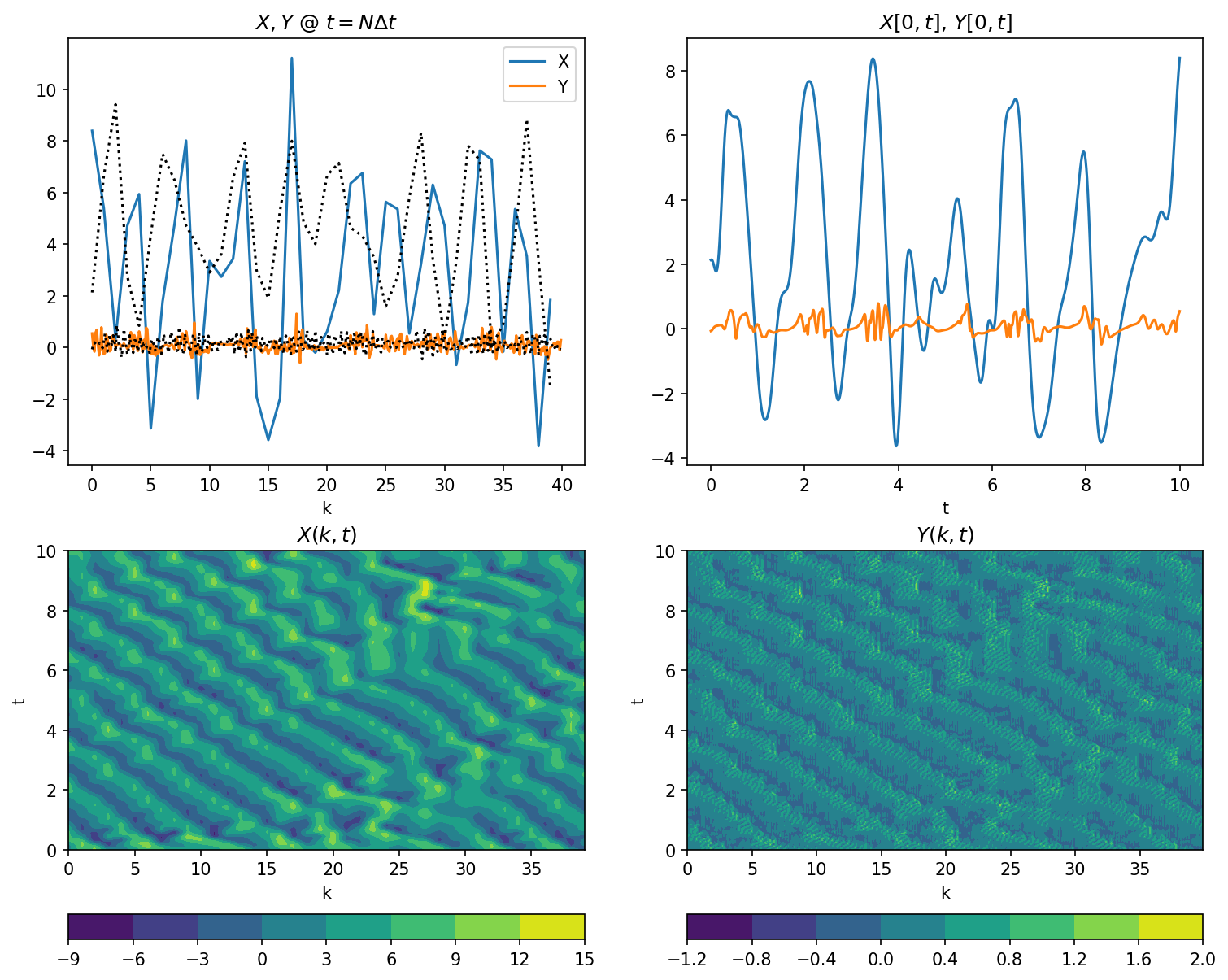
We initialise the L96 two time-scale model using a set of random normally distributed values for \(X\), and zeros for \(Y\), and run it forward for a period ns_spinup to allow the model to spinup. The \(X\) and \(Y\) components of the spinup are then used as initial conditions for another forward run for a time period ns to represent the unobserved truth field from which our observations will be derived.
Note that in reality we do not observe the fine scale components (\(Y\)s) and so this is what we aim to represent in the parameterisation in the GCM() function.
# Set up the "truth" 2-scale L96 model
M_truth = L96(Config.K, Config.J, F=Config.F_truth, dt=Config.dt)
Generate the initial conditions of \(X\) and \(Y\)
M_truth.set_state(rng.standard_normal((Config.K)), 0 * M_truth.j)

# The model runs for `ns_spinup` timesteps to spin-up
X_spinup, Y_spinup, t_spinup = M_truth.run(Config.si, Config.si * Config.ns_spinup)

# The initial conditions for the first forecast (prior to DA)
# are the last time sample after spinup
X_init = X_spinup[-1, :]
Y_init = Y_spinup[-1, :]
Using the generated initial conditions above, run L96 to generate the truth.
M_truth.set_state(X_init, Y_init)
L96: K=40 J=10 F=10 h=1 b=10 c=10 dt=0.005
If given in Config, give F a seasonal cycle in the truth model
if Config.seasonal:
    ann_period = 2000
    mon_period = 100
    mon_per_ann = ann_period / mon_period
    X_truth, Y_truth, t_truth = M_truth.run(Config.si, Config.si * mon_period)
    for i in range(1, int(Config.ns / mon_period)):
        M_truth.set_state(X_truth[-1, ...], Y_truth[-1, ...])
        M_truth.set_param(F=Config.F_truth + 2 * np.sin(2 * np.pi * i / mon_per_ann))
        X_step, Y_step, t_step = M_truth.run(Config.si, Config.si * mon_period)
        X_truth = np.concatenate((X_truth, X_step[1:None, ...]))
        Y_truth = np.concatenate((Y_truth, Y_step[1:None, ...]))
        t_truth = np.concatenate((t_truth, t_truth[-1] + t_step[1:None]))
else:
    X_truth, Y_truth, t_truth = M_truth.run(Config.si, Config.si * Config.ns)
Now, we generate climatological background (temporal) covariance B_clim2 for the 2-scale L96 model.
B_clim2 = np.cov(X_truth.T)
Plotting values of \(X\) and \(Y\)
plt.figure(figsize=(12, 10), dpi=150)
plt.subplot(221)

# Snapshot of X[k]
plt.plot(M_truth.k, X_truth[-1, :], label="X")
plt.plot(M_truth.j / M_truth.J, Y_truth[-1, :], label="Y")
plt.legend()
plt.xlabel("k")
plt.title("$X,Y$ @ $t=N\Delta t$")
plt.plot(M_truth.k, X_truth[0, :], "k:")
plt.plot(M_truth.j / M_truth.J, Y_truth[0, :], "k:")
plt.subplot(222)

# Sample time-series X[0](t), Y[0](t)
plt.plot(t_truth, X_truth[:, 0], label="X")
plt.plot(t_truth, Y_truth[:, 0], label="Y")
plt.xlabel("t")
plt.title("$X[0,t]$, $Y[0,t]$")
plt.subplot(223)

# Full model history of X
plt.contourf(M_truth.k, t_truth, X_truth)
plt.colorbar(orientation="horizontal")
plt.xlabel("k")
plt.ylabel("t")
plt.title("$X(k,t)$")
plt.subplot(224)

# Full model history of Y
plt.contourf(M_truth.j / M_truth.J, t_truth, Y_truth)
plt.colorbar(orientation="horizontal")
plt.xlabel("k")
plt.ylabel("t")
plt.title("$Y(k,t)$");
Generating climatological background covariance B_clim1 for 1-scale L96 model. This climatological covariance will be used by the 3-dimensional variational (3DVar) DA method, or by the hybrid 3DVar-EnKF method. Since we cannot observe every state variable at every possible location, when assimilting sparse observations into the model, we need to use each observation to update multiple model locations, usually around the observed location. The covariance are thus needed to project the model-observation misfits between different model locations in certain DA methods such as 3DVar and EnKF.
M_1s = L96s(Config.K, F=Config.F_truth, dt=Config.dt, method=RK4)
M_1s.set_state(X_init)
X1_truth, t1_truth = M_1s.run(Config.si * Config.ns)
B_clim1 = np.cov(X1_truth.T)
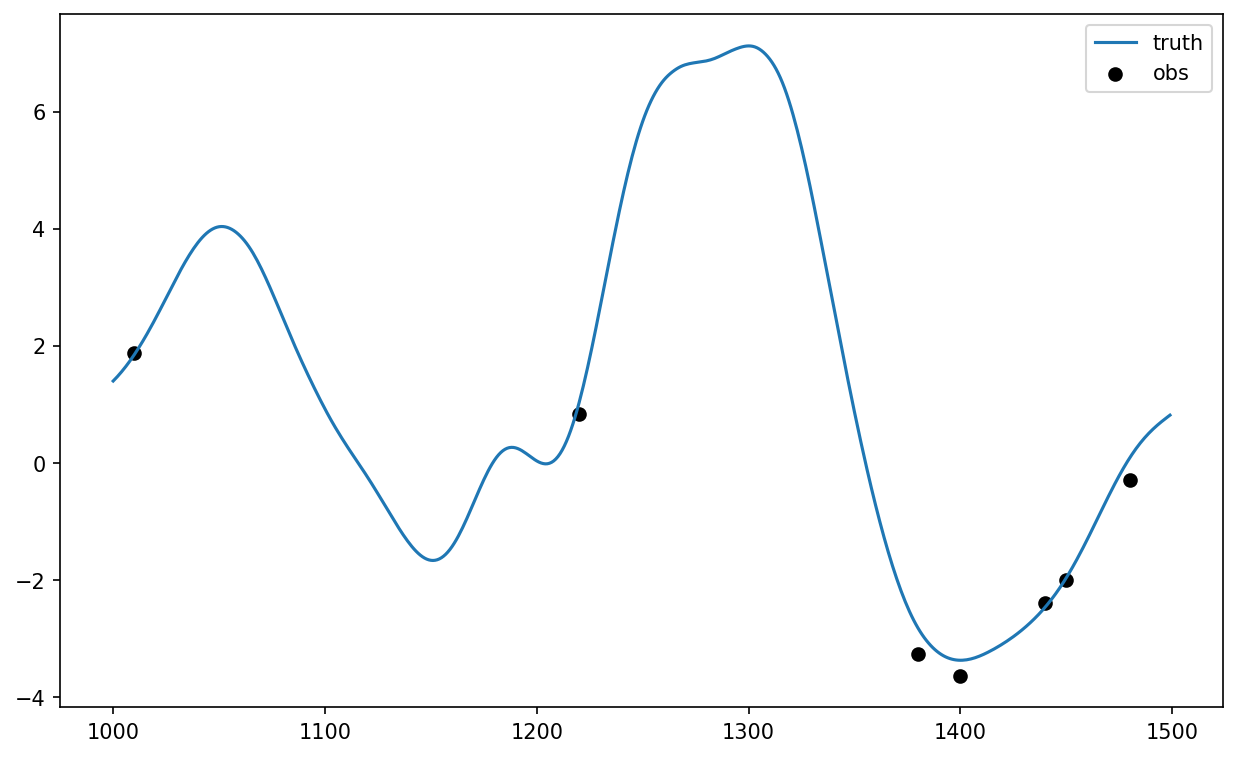
3. Generate synthetic observations#
Here we generate a set of sparse observations by sampling from the X_truth run and adding some random Gaussian noise. The observations are stored as individual samples, each containing the time, location, and value.
# Sample the "truth" to generate observations at certain times (t_obs) and locations (l_obs)
t_obs = np.tile(
    np.arange(Config.obs_freq, Config.ns_da + Config.obs_freq, Config.obs_freq),
    [int(Config.K * Config.obs_density), 1],
).T

l_obs = np.zeros(t_obs.shape, dtype="int")
for i in range(l_obs.shape[0]):
    l_obs[i, :] = rng.choice(
        Config.K, int(Config.K * Config.obs_density), replace=False
    )

X_obs = X_truth[t_obs, l_obs] + Config.obs_sigma * rng.standard_normal(l_obs.shape)
The covariance matrix R for the observations (used to express the uncertainty in the observations during DA) is given as a diagonal matrix with entries defined by the square of the “observational error standard deviation”. \(R\) is a diagonal matrix because we assume that the errors of different observations are independent. The function find_obs is used here to find the locations and values of a set of observations given the observed times.
# Calculated observation covariance matrix, assuming independent observations
R = Config.obs_sigma**2 * np.eye(int(Config.K * Config.obs_density))
plt.figure(figsize=[10, 6], dpi=150)
plt.plot(range(1000, 1500), X_truth[1000:1500, 0], label="truth")
plt.scatter(
    t_obs[100:150, 0],
    DA_methods.find_obs(0, X_obs, t_obs, l_obs, [t_obs[100, 0], t_obs[150, 0]]),
    color="k",
    label="obs",
)
plt.legend();
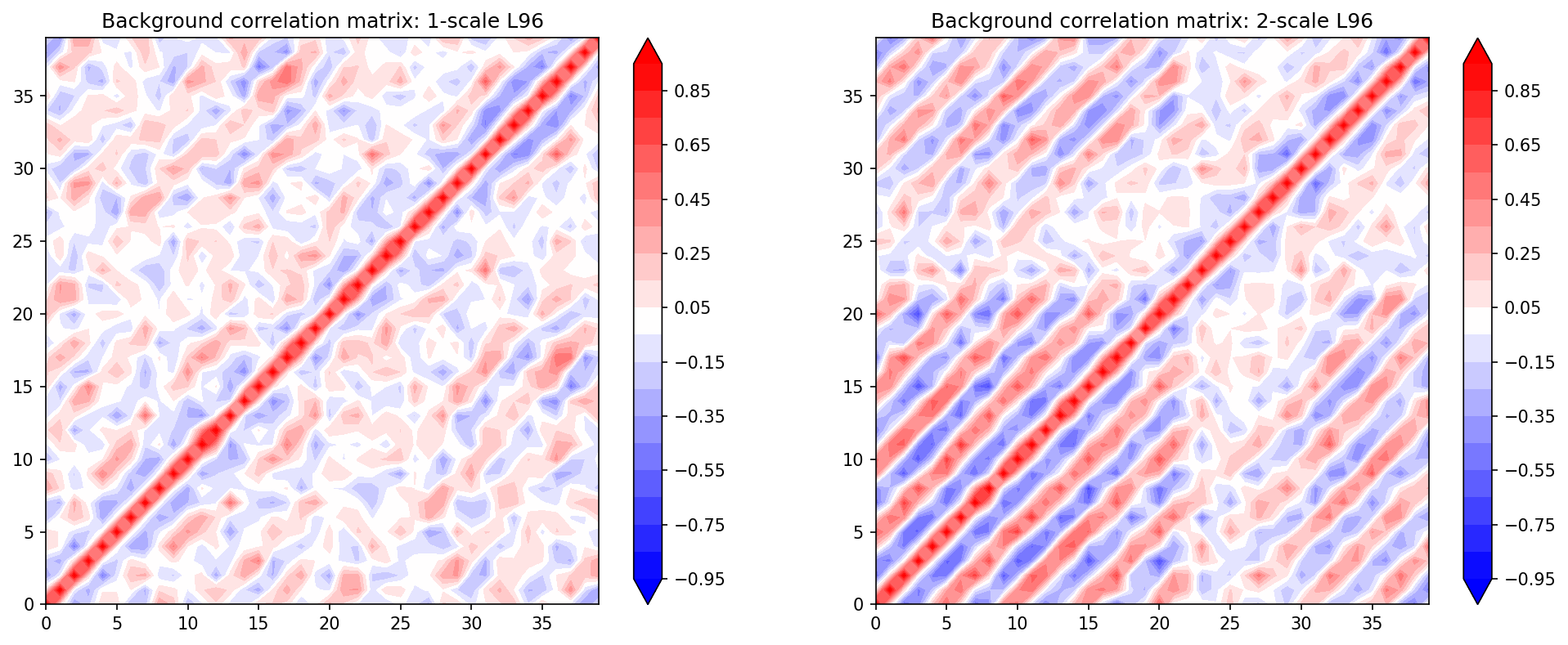
Check the Model Background Covariances for the variable X#
The climatological covariances of both the “truth” (2-scale L96) and “GCM” (1-scale L96) are computed a-priori from a long run.
B_corr1 = np.zeros(B_clim1.shape)
B_corr2 = np.zeros(B_clim2.shape)
for i in range(B_clim1.shape[0]):
    for j in range(B_clim1.shape[1]):
        B_corr1[i, j] = B_clim1[i, j] / np.sqrt(B_clim1[i, i] * B_clim1[j, j])
        B_corr2[i, j] = B_clim2[i, j] / np.sqrt(B_clim2[i, i] * B_clim2[j, j])
plt.figure(figsize=(16, 6), dpi=150)
plt.subplot(121)
plt.contourf(B_corr1, cmap="bwr", extend="both", levels=np.linspace(-0.95, 0.95, 20))
plt.colorbar()
plt.title("Background correlation matrix: 1-scale L96")
plt.subplot(122)
plt.contourf(B_corr2, cmap="bwr", extend="both", levels=np.linspace(-0.95, 0.95, 20))
plt.colorbar()
plt.title("Background correlation matrix: 2-scale L96");
4. Run Data Assimilation#
During each DA cycle, we produce an updated state estimate for all \(K\) grid points, and all n number of ensemble members.
The inputs are:
prior estimate (the forecast at time t for all K grid points, and all n number of ensemble members)
observations (N observations)
operator matrix (N x K)
covariance over obs (N x N)
covariance over model (K x K)
start_time = time.time()

# Set up array to store DA increments
X_inc = np.zeros((int(Config.ns_da / Config.DA_freq), Config.K, Config.nens))
if Config.DA == "3DVar":
    X_inc = np.squeeze(X_inc)

t_DA = np.zeros(int(Config.ns_da / Config.DA_freq))
# Initialize ensemble with perturbations
i_t = 0
ensX = X_init[None, :, None] + rng.standard_normal((1, Config.K, Config.nens))
X_post = ensX[0, ...]
# Localize the covariance matrix in advance to avoid the calculation at each DA step
# The localization weight matrix is also saved for EnKF

B_loc, W_clim = DA_methods.localize_covariance(B_clim1, loc=Config.B_loc)

if Config.param_DA:
    mean_param = np.zeros((int(Config.ns_da / Config.DA_freq), len(Config.GCM_param)))
    spread_param = np.zeros((int(Config.ns_da / Config.DA_freq), len(Config.GCM_param)))
    param_scale = Config.param_sd
    W = np.ones((Config.K + len(Config.GCM_param), Config.K + len(Config.GCM_param)))
    W[0 : Config.K, 0 : Config.K] = W_clim
else:
    W = W_clim
    param_scale = np.zeros(Config.GCM_param.shape)
ens_param = np.zeros((len(Config.GCM_param), Config.nens))
for i in range(len(Config.GCM_param)):
    ens_param[i, :] = Config.GCM_param[i] + rng.normal(
        scale=param_scale[i], size=Config.nens
    )
for cycle in np.arange(0, Config.ns_da / Config.DA_freq, dtype=int):
    # Set up array to store model forecast for each DA cycle
    ensX_fcst = np.zeros((Config.DA_freq + 1, Config.K, Config.nens))

    # Model forecast for next DA cycle
    for n in range(Config.nens):
        ensX_fcst[..., n] = GCM(
            X_post[0 : Config.K, n],
            Config.F_fcst,
            Config.dt,
            Config.DA_freq,
            ens_param[:, n],
        )[0]

    i_t = i_t + Config.DA_freq

    # Get prior/background from the forecast
    X_prior = ensX_fcst[-1, ...]

    # Call DA
    t_DA[cycle] = t_truth[i_t]
    if Config.DA == "EnKF":
        H = DA_methods.observation_operator(Config.K, l_obs, t_obs, i_t)

        # Augment state vector with parameters when doing parameter estimation
        if Config.param_DA:
            H = np.concatenate(
                (H, np.zeros((H.shape[0], len(Config.GCM_param)))), axis=-1
            )
            X_prior = np.concatenate((X_prior, ens_param))
        B_ens = np.cov(X_prior)
        B_ens_loc = B_ens * W
        X_post = DA_methods.EnKF(X_prior, X_obs[t_obs == i_t], H, R, B_ens_loc)

        X_post[0 : Config.K, :] = DA_methods.ens_inflate(
            X_post[0 : Config.K, :],
            X_prior[0 : Config.K, :],
            Config.inflate_opt,
            Config.inflate_factor,
        )

        if Config.param_DA:
            X_post[-len(Config.GCM_param) :, :] = DA_methods.ens_inflate(
                X_post[-len(Config.GCM_param) :, :],
                X_prior[-len(Config.GCM_param) :, :],
                Config.param_inflate,
                Config.param_inf_factor,
            )
            ens_param = X_post[-len(Config.GCM_param) :, :]

    elif Config.DA == "HyEnKF":
        H = DA_methods.observation_operator(Config.K, l_obs, t_obs, i_t)
        B_ens = (
            np.cov(X_prior) * (1 - Config.hybrid_factor)
            + B_clim1 * Config.hybrid_factor
        )
        B_ens_loc = B_ens * W
        X_post = DA_methods.EnKF(X_prior, X_obs[t_obs == i_t], H, R, B_ens_loc)
        X_post = DA_methods.ens_inflate(
            X_post, X_prior, Config.inflate_opt, Config.inflate_factor
        )

    elif Config.DA == "3DVar":
        X_prior = np.squeeze(X_prior)
        H = DA_methods.observation_operator(Config.K, l_obs, t_obs, i_t)
        X_post = DA_methods.Lin3dvar(X_prior, X_obs[t_obs == i_t], H, R, B_loc, 3)

    elif Config.DA == "Replace":
        X_post = X_prior
        X_post[l_obs[t_obs == i_t]] = X_obs[t_obs == i_t]

    elif Config.DA == "None":
        X_post = X_prior

    if not Config.DA == "None":
        # Get current increments
        X_inc[cycle, ...] = (
            np.squeeze(X_post[0 : Config.K, ...]) - X_prior[0 : Config.K, ...]
        )

        # Get posterior info about the estimated parameters
        if Config.param_DA:
            mean_param[cycle, :] = ens_param.mean(axis=-1)
            spread_param[cycle, :] = ens_param.std(axis=-1)

    # Reset initial conditions for next DA cycle
    ensX_fcst[-1, :, :] = X_post[0 : Config.K, :]
    ensX = np.concatenate((ensX, ensX_fcst[1:None, ...]))

print(f"Time to complete DA: {round(time.time() - start_time, 2)} (s)")
Time to complete DA: 35.82 (s)
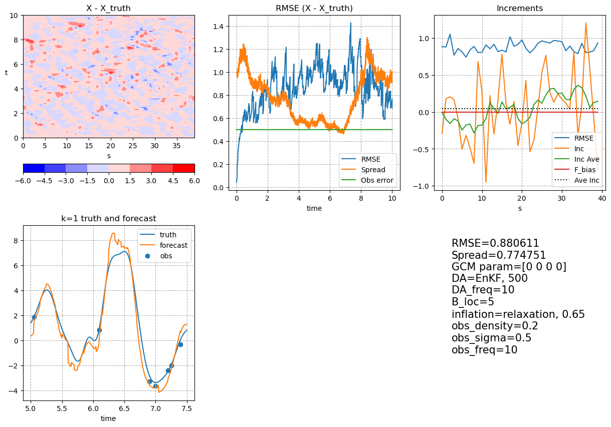
5. Post Processing and Visualization#
mean_X = np.mean(ensX, axis=-1)
clim = np.max(np.abs(mean_X - X_truth[0 : (Config.ns_da + 1), :]))
fig, axes = plt.subplots(2, 3, figsize=(15, 10))
ch = axes[0, 0].contourf(
    M_truth.k,
    t_truth[0 : (Config.ns_da + 1)],
    mean_X - X_truth[0 : (Config.ns_da + 1), :],
    cmap="bwr",
    vmin=-clim,
    vmax=clim,
    extend="neither",
)

plt.colorbar(ch, ax=axes[0, 0], orientation="horizontal")
axes[0, 0].set_xlabel("s")
axes[0, 0].set_ylabel("t", rotation=0)
axes[0, 0].set_title("X - X_truth")

axes[0, 1].plot(
    t_truth[0 : (Config.ns_da + 1)],
    np.sqrt(((mean_X - X_truth[0 : (Config.ns_da + 1), :]) ** 2).mean(axis=-1)),
    label="RMSE",
)
axes[0, 1].plot(
    t_truth[0 : (Config.ns_da + 1)],
    np.mean(np.std(ensX, axis=-1), axis=-1),
    label="Spread",
)
axes[0, 1].plot(
    t_truth[0 : (Config.ns_da + 1)],
    Config.obs_sigma * np.ones((Config.ns_da + 1)),
    label="Obs error",
)
axes[0, 1].legend()
axes[0, 1].set_xlabel("time")
axes[0, 1].set_title("RMSE (X - X_truth)")
axes[0, 1].grid(which="both", linestyle="--")

axes[0, 2].plot(
    M_truth.k,
    np.sqrt(((mean_X - X_truth[0 : (Config.ns_da + 1), :]) ** 2).mean(axis=0)),
    label="RMSE",
)
X_inc_ave = X_inc / Config.DA_freq / Config.si
axes[0, 2].plot(M_truth.k, X_inc_ave.mean(axis=(0, -1)), label="Inc")
axes[0, 2].plot(
    M_truth.k,
    DA_methods.running_average(X_inc_ave.mean(axis=(0, -1)), 7),
    label="Inc Ave",
)
axes[0, 2].plot(
    M_truth.k,
    np.ones(M_truth.k.shape) * (Config.F_fcst - Config.F_truth),
    label="F_bias",
)
axes[0, 2].plot(
    M_truth.k,
    np.ones(M_truth.k.shape) * (X_inc / Config.DA_freq / Config.si).mean(),
    "k:",
    label="Ave Inc",
)
axes[0, 2].legend()
axes[0, 2].set_xlabel("s")
axes[0, 2].set_title("Increments")
axes[0, 2].grid(which="both", linestyle="--")

plot_start, plot_end = 1000, 1500
plot_start_DA, plot_end_DA = int(plot_start / Config.DA_freq), int(
    plot_end / Config.DA_freq
)
plot_x = 0

axes[1, 0].plot(
    t_truth[plot_start:plot_end], X_truth[plot_start:plot_end, plot_x], label="truth"
)
axes[1, 0].plot(
    t_truth[plot_start:plot_end], mean_X[plot_start:plot_end, plot_x], label="forecast"
)
axes[1, 0].scatter(
    t_DA[plot_start_DA - 1 : plot_end_DA - 1],
    DA_methods.find_obs(plot_x, X_obs, t_obs, l_obs, [plot_start, plot_end]),
    label="obs",
)
axes[1, 0].grid(which="both", linestyle="--")
axes[1, 0].set_xlabel("time")
axes[1, 0].set_title("k=" + str(plot_x + 1) + " truth and forecast")
axes[1, 0].legend()

if Config.param_DA:
    for i, c in zip(np.arange(len(Config.GCM_param), 0, -1), ["r", "b", "g", "k"]):
        axes[1, 1].plot(
            t_DA,
            DA_methods.running_average(mean_param[:, i - 1], 100),
            c + "-",
            label="C{} {:3f}".format(
                i - 1, mean_param[int(len(t_DA) / 2) :, i - 1].mean()
            ),
        )
        axes[1, 1].plot(
            t_DA,
            DA_methods.running_average(
                mean_param[:, i - 1] + spread_param[:, i - 1], 100
            ),
            c + ":",
            label=f"SD {spread_param[int(len(t_DA) / 2):, i - 1].mean():3f}",
        )
        axes[1, 1].plot(
            t_DA,
            DA_methods.running_average(
                mean_param[:, i - 1] - spread_param[:, i - 1], 100
            ),
            c + ":",
        )
    axes[1, 1].legend()
    axes[1, 1].grid(which="both", linestyle="--")

else:
    axes[1, 1].axis("off")

axes[1, 2].text(
    0.1,
    0.2,
    (
        f"RMSE={np.sqrt(((mean_X - X_truth[0 : (Config.ns_da + 1), :]) ** 2).mean()):3f}\n"
        f"Spread={np.mean(np.std(ensX, axis=-1)):3f}\n"
        f"GCM param={Config.GCM_param}\n"
        f"DA={Config.DA}, {Config.nens}\n"
        f"DA_freq={Config.DA_freq}\n"
        f"B_loc={Config.B_loc}\n"
        f"inflation={Config.inflate_opt}, {Config.inflate_factor}\n"
        f"obs_density={Config.obs_density}\n"
        f"obs_sigma={Config.obs_sigma}\n"
        f"obs_freq={Config.obs_freq}\n"
    ),
    fontsize=15,
)
axes[1, 2].axis("off")

if Config.save_fig:
    output_dir = os.path.join(".", "DA_data")
    os.makedirs(output_dir, exist_ok=True)
    exp_number = np.random.randint(1, 10000)
    with open(os.path.join(output_dir, f"config_{exp_number}.txt"), "w") as f:
        f.write(
            output_dir
            + str({k: v for k, v in Config.__dict__.items() if not k.startswith("_")})
        )
    plt.savefig(os.path.join(output_dir, f"fig_{exp_number}.png"))
Save DA output for further analysis
if Config.save_data:
    output_filename = (
        f"K_{Config.K}_"
        f"J_{Config.J}_"
        f"obs_freq_{Config.obs_freq}_"
        f"F_truth_{Config.F_truth}_"
        f"F_fcst_{Config.F_fcst}_"
        f"ns_da_{Config.ns_da}_"
        f"ns_{Config.ns}_"
        f"ns_spinup_{Config.ns_spinup}_"
        f"dt_{Config.dt}_"
        f"si_{Config.si}_"
        f"B_loc_{Config.B_loc}_"
        f"DA_{Config.DA}_"
        f"nens_{Config.nens}_"
        f"inflate_opt_{Config.inflate_opt}_"
        f"inflate_factor_{Config.inflate_factor}_"
        f"hybrid_factor_{Config.hybrid_factor}_"
        f"obs_density_{Config.obs_density}_"
        f"DA_freq_{Config.DA_freq}_"
        f"obs_sigma_{Config.obs_sigma}.npz"
    )
    output_dir = os.path.join(".", "DA_data")
    os.makedirs(output_dir, exist_ok=True)
    np.savez(
        os.path.join(output_dir, output_filename),
        mean_X=mean_X,
        X_truth=X_truth,
        X_inc_ave=X_inc_ave,
    )