Interpreting Neural Networks

Outline

Neural networks are great at approximating complex functions, but usually provide little direct insight or interpretation into the functional relationships that are approximated. In this notebook we present some techniques that can be used to probe neural networks and indirectly infer what the network has learnt.

We present two class of approaches: feature importance and saliency maps.

Set up the model and networks

import numpy as np
import math

import torch
from torch.autograd import Variable, grad
from torch.autograd.functional import jacobian
import torch.nn.functional as F
import torch.utils.data as Data
from torch import nn, optim

from sklearn.metrics import r2_score
from sklearn.linear_model import LinearRegression


import matplotlib.pyplot as plt

from L96_model import (
    L96,
    L96_eq1_xdot,
    integrate_L96_2t,
    EulerFwd,
    RK2,
    RK4,
)

%matplotlib inline

np.random.seed(14)  # For reproducibility
torch.manual_seed(14)  # For reproducibility

<torch._C.Generator at 0x7f31de8bba90>

# create a confusion matrix like figure
def imshow(x, colorbar_pct=97.5, cmap="seismic", label=None, vlim=None, **kw):
    if vlim is None:
        vlim = np.percentile(np.abs(x), colorbar_pct)
    plt.xlabel("Input dimension", fontsize=14)
    plt.ylabel("Output dimension", fontsize=14)
    plt.xticks(range(8))
    plt.yticks(range(8))
    im = plt.imshow(x, vmin=-vlim, vmax=vlim, cmap=cmap, **kw)
    cb = plt.colorbar()
    if label is not None:
        cb.set_label(label, fontsize=14)
    return im


def plot_feature_importance(result, feature_index):
    fig = plt.figure()
    ax = fig.add_axes([0, 0, 1, 1])
    ax.set_xlabel("Shift in score")
    ax.set_ylabel("Column")
    ax.set_title("Permutation Feature Importance for k=" + str(feature_index))

    predictors = result[:, 0]
    scores = result[:, 1]
    y_pos = range(len(predictors))

    ax.barh(y_pos, scores)
    plt.yticks(y_pos, predictors)
    plt.show()

Generate L96 data

time_steps = 20000
Forcing, dt, T = 18, 0.01, 0.01 * time_steps

# Create a "synthetic world" with K=8 and J=32
K = 8
J = 32
W = L96(K, J, F=Forcing)
# Get training data for the neural network.

# - Run the true state and output subgrid tendencies (the effect of Y on X is xytrue):
X_true, _, _, xy_true = W.run(dt, T, store=True, return_coupling=True)

Load a pretrained neural network

# Specify a path
PATH = "networks/network_3_layers_100_epoches.pth"
# Load
weights = torch.load(PATH)

class Net_ANN(nn.Module):
    def __init__(self):
        super(Net_ANN, self).__init__()
        self.linear1 = nn.Linear(8, 16)  # 8 inputs, 16 neurons for first hidden layer
        self.linear2 = nn.Linear(16, 16)  # 16 neurons for second hidden layer
        self.linear3 = nn.Linear(16, 8)  # 8 outputs

    def forward(self, x):
        x = x.to(self.linear1.weight.dtype)
        x = F.relu(self.linear1(x))
        x = F.relu(self.linear2(x))
        x = self.linear3(x)
        return x

model = Net_ANN()
model.load_state_dict(weights)
model.eval()

Net_ANN(
  (linear1): Linear(in_features=8, out_features=16, bias=True)
  (linear2): Linear(in_features=16, out_features=16, bias=True)
  (linear3): Linear(in_features=16, out_features=8, bias=True)
)

Feature importance

Feature importance is a simple technique that allows us to identify the contribution that each input feature has towards bringing a neural network’s output close to the target (reducing the loss or performing well on some skill metric).

In this process the importance of each input feature is evaluate by scrambling its value and evaluating how much the network output changed in response. This changed output is compared to the target, to see whether the particular input has small or large effect on the network output.

# First we compute the baeline score (how the model does with original data)
feature_index = 3  # which k do we focus on for output.
baseline_r2 = r2_score(
    model(torch.tensor(X_true)).detach().numpy()[:, feature_index],
    xy_true[:, feature_index],
)

scrambled_r2 = []
for column in range(X_true.shape[1]):
    # Create a copy of X_test
    X_copy = X_true.copy()

    # Scramble the values of the given predictor
    shuffle_col = X_copy[:, column]
    np.random.shuffle(shuffle_col)
    X_copy[:, column] = shuffle_col

    # Calculate the new R2
    score = r2_score(
        model(torch.tensor(X_copy)).detach().numpy()[:, feature_index],
        xy_true[:, feature_index],
    )

    # Append the increase in R2 to the list of results
    scrambled_r2.append([column, abs(score - baseline_r2)])

# Put the results into a pandas dataframe and rank the predictors by score
scrambled_r2 = np.array(scrambled_r2)

plot_feature_importance(scrambled_r2, feature_index)

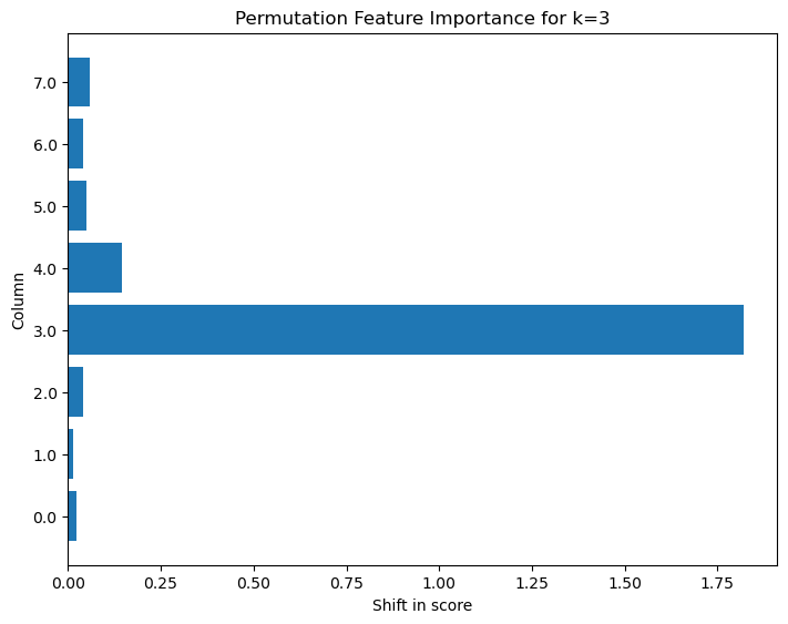
Notice above that that we are considering the impact that shuffling the inputs has on a particular output feature ( feature index). The plot below shows that for this network the largest deterioration in model skill takes place when the input feature at the same k as the output k is varied, suggesting the local behavior of the dependence between the inputs and outputs.

Saliency maps

Saliency maps are popular visualization techniques for gaining insights on why neural networks made a particular decision on the given input data. They are usually rendered as a heatmap, where hotness corresponds to regions that have a big impact on the model’s final decision. They are helpful, for example, when you are frustrated by your model incorrectly classifying a certain datapoint, because you can look at the input features that led to that decision [Simonyan et al., 2013], [Baehrens et al., 2010], [Adebayo et al., 2018].

In this notebook, we will explore the different ways one could render saliency maps for the L96 data and visualize them.

Generate saliency maps using input gradients

Since neural networks are differentiable, the simplest way of generating saliency maps (i.e. a quantification of the sensitivity of the output to the input) is to just take its first derivative with respect to its inputs (or Jacobian, for networks with multiple inputs and outputs).

We can do this easily in Pytorch using torch.autograd.functional.jacobian.

Full Jacobian method

%%time
jacobians = np.array(
    [
        jacobian(
            model,
            torch.tensor(np.single(X_true[i, :]), requires_grad=True),
            create_graph=False,
        )
        .detach()
        .numpy()
        for i in range(200)
    ]
)

CPU times: user 244 ms, sys: 23 µs, total: 244 ms
Wall time: 204 ms

This gives us an array of 8x8 gradients, one for each of 200 input samples. Let’s visualize their average value, as well as their standard deviation:

fig = plt.figure(figsize=(12, 4))
fig.suptitle(
    "Mean and standard deviation of NN input gradients across the dataset",
    fontsize=18,
    y=1.025,
)

plt.subplot(121)
plt.title("Average value", fontsize=16)
imshow(jacobians.mean(0), label="Average input derivative", vlim=0.85)

plt.subplot(122)
plt.title("Standard deviation", fontsize=16)
imshow(jacobians.std(0), label="Standard deviation", vlim=0.85)

plt.show()

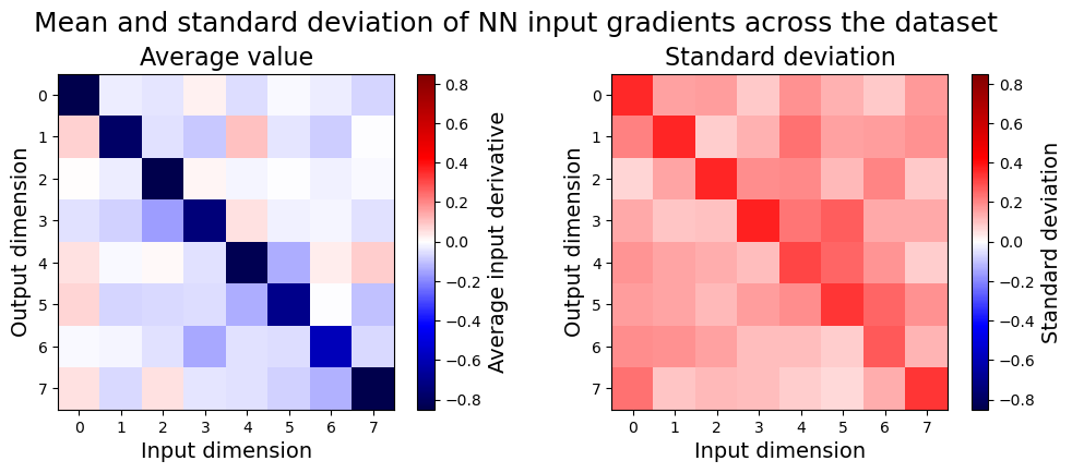
The dominant term in the average gradient is close to -1 along the main diagonal, but there are significant off-diagonal elements, and also significant deviation across samples. It’s interesting to compare this to the behavior of a linear regression model:

Create and fit a Linear Regression model

lr = LinearRegression()
lr.fit(X_true, xy_true)

plt.title("Comparing to linear model", fontsize=16)
imshow(lr.coef_, label="Linear regression weight", vlim=0.85)
plt.show()

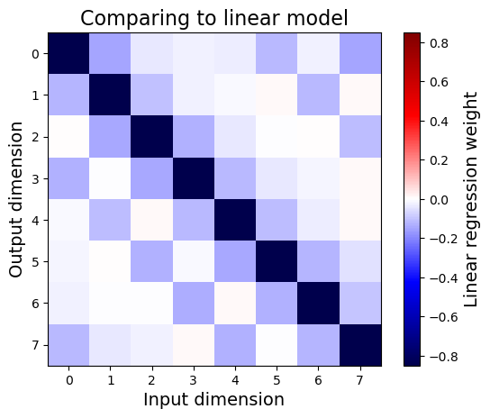
We see that the weights of a linear regression model generally match the average input gradients of the neural network, especially down the main diagonal. This makes some sense given that, at each point, input gradients represent the best local linear model that approximates the nonlinear neural network.

Although computing full Jacobians works fine for a small example, it can become expensive for large networks and input/output dimensions, so we can also approximate it using finite differences:

Approximate Jacobian method

%%time
epsilon = 1e-2
approx_jacobians = []

for case in range(200):
    inputs = X_true[case, :].copy()
    inputs = torch.tensor(np.single(inputs), requires_grad=False)
    pred = model(inputs)
    Js = np.zeros((len(inputs), len(pred)))
    for j in range(len(inputs)):
        perturb = np.zeros_like(inputs)
        perturb[j] = epsilon
        inputs_perturbed = (inputs + perturb).clone().detach().requires_grad_(False)
        Js[j, :] = (
            model(inputs_perturbed).detach().numpy() - pred.detach().numpy()
        ) / epsilon
    approx_jacobians.append(Js.T)

approx_jacobians = np.array(approx_jacobians)

CPU times: user 229 ms, sys: 112 µs, total: 230 ms
Wall time: 230 ms

(Technically this is slightly slower than the previous example, but it can be more performant for large networks.)

Let’s see how that looks:

plt.title("Interpreting the network with finite differences", fontsize=16)
imshow(approx_jacobians.mean(0), label="Average finite difference")
plt.show()

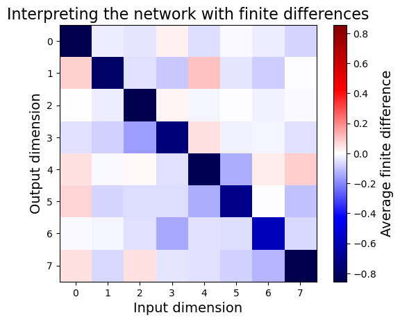
As expected, it’s fairly similar to the full Jacobian method.

Generate saliency maps layerwise relevance propagation (LRP)

Another proposed method for generating saliency maps is [Bach et al., 2015]. With a baseline of 0, this method is akin to multiplying the input gradients by the input itself (per [Ancona et al., 2018]), but it has become popular in the climate community and does support alternative baselines.

for name in weights.keys():
    print(name)

linear1.weight
linear1.bias
linear2.weight
linear2.bias
linear3.weight
linear3.bias

epsilon = 0.0  # filtering small values
gamma = 0.0  # give more weights to positive values

## get the weight and bias of the NN
def get_weight(weightsname):
    Ws = []
    Bs = []
    for i, name in enumerate(weights.keys()):
        if i % 2 == 0:
            Ws.append(np.array(weights[name]))
        else:
            Bs.append(np.array(weights[name]))
    return Ws, Bs  # weights and biases


# forward pass to calculate the output of each layer
def forward_pass(data, Ws, Bs):
    L = len(Ws)
    forward = [data] + [None] * L

    for l in range(L - 1):
        forward[l + 1] = np.maximum(0, Ws[l].dot(forward[l])) + Bs[l]  # ativation ReLu

    ## for last layer that does not have activation function
    forward[L] = Ws[L - 1].dot(forward[L - 1]) + Bs[L - 1]  # linear last layer
    return forward


def rho(w, l):
    w_intermediate = w + [0.0, 0.0, 0.0, 0.0, 0.0][l] * np.maximum(0, w)
    return w_intermediate + gamma * np.maximum(0, w_intermediate)


def incr(z, l):
    return z + [0.0, 0.0, 0.0, 0.0, 0.0][l] * (z**2).mean() ** 0.5 + 1e-9

## backward pass to compute the LRP of each layer. Same rule applied to the first layer (input layer)
def onelayer_LRP(W, B, forward, nz, zz):
    mask = np.zeros((nz))
    mask[zz] = 1
    L = len(W)
    R = [None] * L + [forward[L] * mask]  # start from last layer Relevance

    for l in range(0, L)[::-1]:
        w = rho(W[l], l)
        b = rho(B[l], l)
        z = incr(w.dot(forward[l]) + b + epsilon, l)  # step 1 - forward pass
        s = np.array(R[l + 1]) / np.array(z)  # step 2 - element-wise division
        c = w.T.dot(s)  # step 3 - backward pass
        R[l] = forward[l] * c  # step 4 - element-wise product
    return R


def LRP_alllayer(data, weights):
    """inputs:
        data: for single sample, with the right asix, the shape is (nz,naxis)
        weights: dictionary of weights and biases
    output:
        LRP, shape: (nx,L+1) that each of the column consist of L+1 array
        Relevance of fisrt layer's pixels"""
    nx = data.shape[0]
    ## step 1: get the wieghts
    Ws, Bs = get_weight(weights)

    ## step 2: call the forward pass to get the intermediate layers output
    inter_layer = forward_pass(data, Ws, Bs)

    ## loop over all z and get the LRP of each layer
    R_all = [None] * nx
    relevance = np.zeros((nx, nx))
    for xx in range(nx):
        R_all[xx] = onelayer_LRP(Ws, Bs, inter_layer, nx, xx)
        relevance[xx, :] = R_all[xx][0]

    return np.array(R_all, dtype=object), relevance

%%time
R_many = []
for case in range(200):
    inputs = np.copy(X_true[case, :])
    _, Rs = LRP_alllayer(inputs, weights)
    R_many.append(Rs)
LRP = np.stack(R_many)

CPU times: user 139 ms, sys: 268 µs, total: 139 ms
Wall time: 139 ms

plt.title("Interpreting the network with\nlayerwise relevance propagation", fontsize=16)
imshow(LRP.mean(0), label="Average LRP")
plt.show()

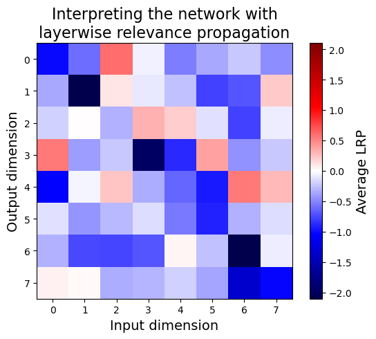
LRP outputs something qualitatively different from the gradient-based methods, and in fact each element should be interpreted more as an attribution score (i.e. the actual contribution of an input to the output) than as a sensitivity score (i.e. how much an output changes with an input). Below, we’ll see that this approximately reduces to multiplying the gradient by the input.

Comparing all of the methods

Let’s look at the output of these methods side-by-side:

comparisons = [
    (jacobians, "Jacobian (exact)"),
    (approx_jacobians, "Jacobian (finite diff)"),
    (LRP, "LRP"),
    (jacobians * X_true[:200][:, np.newaxis, :], "Jacobian * input"),
]

fig = plt.figure(figsize=(10, 8))
fig.suptitle(
    "Comparing average outputs of saliency methods", fontsize=20, y=1.0, va="bottom"
)

for i, (saliency, label) in enumerate(comparisons):
    plt.subplot(2, 2, i + 1)
    plt.title(label, fontsize=16)
    imshow(saliency.mean(0), label=label)

plt.tight_layout()
plt.show()

As expected, LRP and Jacobian * input produce very similar outputs. For more information on the intricacies of saliency maps, see [Ancona et al., 2018] and [Bach et al., 2015].

Summary

In this notebook we introduced some approaches that can be used to better understand how neural networks estimate the output from a given input. This is an important area of research, as we would want to test that the neural networks are producing the right answers for the right reasons (physically reasonable models). This becomes particularly important when we want our networks to produce accurate results (extrapolate) for inputs that were not observed in training data.

In the next notebook we show how physics based constraints can be incorporated into neural networks, in an attempt to further guide the neural network to learn more appropriate relationships between inputs and outputs.