Applying SINDy equation identification to L96#
Outline#
This notebook provides an example of SINDy equation identification in application to the two-scale L96 model with the use of pysindy library. The objective is to try to identify the governing ODEs for the large-scale variable (\(X_i\)) if we know only their time measurements. In other words, we want to see how well the SINDy model can capture the form of the governing equations for large-scale variables in the presence of the subgrid forcing by small-scale variables (\(Y\)) when there is no measurements of the small scales.
Import#
import numpy as np
import pysindy as ps
import matplotlib.pyplot as plt
import seaborn as sns
from L96_model import L96, L96_eq1_xdot, integrate_L96_2t, integrate_L96_1t
Routines for plotting#
colors = [
    "#1f77b4",
    "#ff7f0e",
    "#2ca02c",
    "#d62728",
    "#9467bd",
    "#8c564b",
    "#e377c2",
    "#7f7f7f",
    "#bcbd22",
    "#17becf",
]
def plot_coefficients(
    coefficients, input_features=None, feature_names=None, ax=None, **heatmap_kws
):
    if input_features is None:
        input_features = [f"$\dot x_{k}$" for k in range(coefficients.shape[0])]
    else:
        input_features = [f"$\dot {fi}$" for fi in input_features]

    if feature_names is None:
        feature_names = [f"f{k}" for k in range(coefficients.shape[1])]

    with sns.axes_style(style="white", rc={"axes.facecolor": (0, 0, 0, 0)}):
        if ax is None:
            fig, ax = plt.subplots(1, 1)

        max_mag = np.max(np.abs(coefficients))
        heatmap_args = {
            "xticklabels": input_features,
            "yticklabels": feature_names,
            "center": 0.0,
            "cmap": sns.color_palette("vlag", n_colors=20, as_cmap=True),
            "ax": ax,
            "linewidths": 0.1,
            "linecolor": "whitesmoke",
        }
        heatmap_args.update(**heatmap_kws)

        sns.heatmap(coefficients.T, **heatmap_args)

        ax.tick_params(axis="y", rotation=0)

    return ax
def signed_sqrt(x):
    return np.sign(x) * np.sqrt(np.abs(x))
def compare_coefficient_plots(coefficients, input_features=None, feature_names=None):
    n_cols = len(coefficients)
    with sns.axes_style(style="white", rc={"axes.facecolor": (0, 0, 0, 0)}):
        max_mag = np.max(np.abs(coefficients))
        fig, axs = plt.subplots(1, 1, figsize=(4, 4), sharey=True, sharex=True)
        plot_coefficients(
            signed_sqrt(coefficients),
            input_features=input_features,
            feature_names=feature_names,
            ax=axs,
            cbar=False,
            vmax=max_mag,
            vmin=-max_mag,
        )
        fig.tight_layout()
L96 two-scale model#

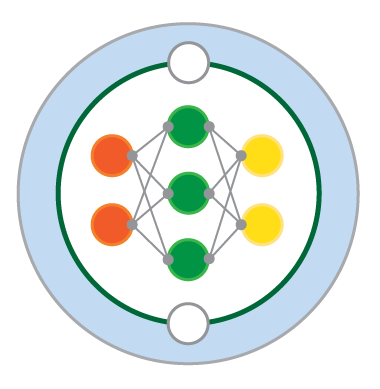
Fig. 7 Visualisation of a two-scale Lorenz ‘96 system with J = 8 and K = 6. Global-scale variables (\(X_k\)) are updated based on neighbouring variables and on the local-scale variables (\(Y_{j,k}\)) associated with the corresponding global-scale variable. Local-scale variabless are updated based on neighbouring variables and the associated global-scale variable. The neighbourhood topology of both local and global-scale variables is circular. Image from Exploiting the chaotic behaviour of atmospheric models with reconfigurable architectures - Scientific Figure on ResearchGate..#
Two-time-scale Lorenz 96 model: $\( \frac{d}{dt} X_k = - X_{k-2} X_{k-1} + X_{k-1} X_{k+1} - X_k + F - \left( \frac{hc}{b} \right) \sum_{j=0}^{J-1} Y_{j,k} \)\( \)\( \frac{d}{dt} Y_{j,k} = - c b Y_{j+1,k} (Y_{j+2,k} - Y_{j-1,k}) - c Y_{j,k} + \left( \frac{hc}{b} \right) \sum_{j=0}^{J-1} X_{k} \)$
We will put K=8 large-scale variables (\(X\)), for each of them there is J=32 small-scale variables (\(Y\)). For the first example, we will consider the case of weak interaction between the scales, which is defined by the parameter \(h\) in the L96 class.
K = 8  # Number of degrees of freedom for X
J = 32  # Number of degrees of freedom for Y per X
Forcing = 18.0  # Model parameter
h = 0.1  # WEAK coupling
def s(k, K):
    """A non-dimension coordinate from -1..+1 corresponding to k=0..K"""
    return 2 * (0.5 + k) / K - 1
# Initial conditions
k = np.arange(K)  # For coordinate in plots
j = np.arange(J * K)  # For coordinate in plots
# Initial conditions
X_init = s(k, K) * (s(k, K) - 1) * (s(k, K) + 1)
Y_init = 0 * s(j, J * K) * (s(j, J * K) - 1) * (s(j, J * K) + 1)
steps = 1000
dt = 0.005
# Create a "real world" with K=8 and J=32
W = L96(K, J, F=Forcing, h=h)
W.set_state(X_init, Y_init)
# Run the true state
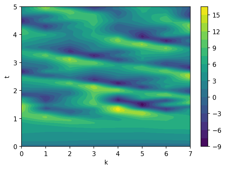
X, Y, t = W.run(dt, dt * steps, store=True)
fig, ax = plt.subplots(1, 1, figsize=(6, 4), dpi=150)
contours = ax.contourf(k, t, X, levels=20)
fig.colorbar(contours)
ax.set(xlabel="k", ylabel="t")
plt.show();
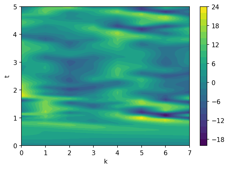
The data array \(X\) will be used for the system identification by SINDy method. We suppose that we do not dispose measurements for the small-scale variables \(Y\), so their contribution to the large-scale dymanics will basically treated as noise.
Define SINDy model#
The goal is to identify the governing equations for the large-scale variables \(X\), having the measurement for them.
differentiation_method = ps.SINDyDerivative(kind="finite_difference", k=1)
feature_library = ps.PolynomialLibrary(degree=2)
# sequential thresholded least squares optimizer
optimizer = ps.STLSQ(threshold=0.3)
model = ps.SINDy(
    differentiation_method=differentiation_method,
    feature_library=feature_library,
    optimizer=optimizer,
    feature_names=[("x" + str(i)) for i in k],
)
Optimize coefficients#
model.fit(X, t=t)
SINDy(differentiation_method=SINDyDerivative(k=1, kind='finite_difference'),
      feature_library=PolynomialLibrary(),
      feature_names=['x0', 'x1', 'x2', 'x3', 'x4', 'x5', 'x6', 'x7'],
      optimizer=STLSQ(threshold=0.3))
In a Jupyter environment, please rerun this cell to show the HTML representation or trust the notebook. On GitHub, the HTML representation is unable to render, please try loading this page with nbviewer.org.
SINDy(differentiation_method=SINDyDerivative(k=1, kind='finite_difference'),
      feature_library=PolynomialLibrary(),
      feature_names=['x0', 'x1', 'x2', 'x3', 'x4', 'x5', 'x6', 'x7'],
optimizer=STLSQ(threshold=0.3))PolynomialLibrary()
PolynomialLibrary()
STLSQ(threshold=0.3)
STLSQ(threshold=0.3)
feature_names = feature_library.get_feature_names()
print(feature_names)
['1', 'x0', 'x1', 'x2', 'x3', 'x4', 'x5', 'x6', 'x7', 'x0^2', 'x0 x1', 'x0 x2', 'x0 x3', 'x0 x4', 'x0 x5', 'x0 x6', 'x0 x7', 'x1^2', 'x1 x2', 'x1 x3', 'x1 x4', 'x1 x5', 'x1 x6', 'x1 x7', 'x2^2', 'x2 x3', 'x2 x4', 'x2 x5', 'x2 x6', 'x2 x7', 'x3^2', 'x3 x4', 'x3 x5', 'x3 x6', 'x3 x7', 'x4^2', 'x4 x5', 'x4 x6', 'x4 x7', 'x5^2', 'x5 x6', 'x5 x7', 'x6^2', 'x6 x7', 'x7^2']
model.print()
(x0)' = 17.900 1 + -1.019 x0 + 0.998 x1 x7 + -0.998 x6 x7
(x1)' = 17.980 1 + -1.026 x1 + 1.000 x0 x2 + -0.999 x0 x7
(x2)' = 17.996 1 + -1.020 x2 + -0.999 x0 x1 + 0.999 x1 x3
(x3)' = 17.992 1 + -1.023 x3 + -1.001 x1 x2 + 1.000 x2 x4
(x4)' = 17.948 1 + -1.022 x4 + -1.000 x2 x3 + 1.000 x3 x5
(x5)' = 17.949 1 + -1.017 x5 + -1.001 x3 x4 + 1.000 x4 x6
(x6)' = 18.009 1 + -1.016 x6 + -1.001 x4 x5 + 0.999 x5 x7
(x7)' = 17.951 1 + -1.016 x7 + 0.998 x0 x6 + -0.998 x5 x6
model.score(X, t=t[1] - t[0])
0.9999919207350484
model.coefficients()
array([[17.90003772, -1.01862501,  0.        ,  0.        ,  0.        ,
         0.        ,  0.        ,  0.        ,  0.        ,  0.        ,
         0.        ,  0.        ,  0.        ,  0.        ,  0.        ,
         0.        ,  0.        ,  0.        ,  0.        ,  0.        ,
         0.        ,  0.        ,  0.        ,  0.99829818,  0.        ,
         0.        ,  0.        ,  0.        ,  0.        ,  0.        ,
         0.        ,  0.        ,  0.        ,  0.        ,  0.        ,
         0.        ,  0.        ,  0.        ,  0.        ,  0.        ,
         0.        ,  0.        ,  0.        , -0.99760226,  0.        ],
       [17.97958814,  0.        , -1.02560838,  0.        ,  0.        ,
         0.        ,  0.        ,  0.        ,  0.        ,  0.        ,
         0.        ,  0.9995848 ,  0.        ,  0.        ,  0.        ,
         0.        , -0.99916774,  0.        ,  0.        ,  0.        ,
         0.        ,  0.        ,  0.        ,  0.        ,  0.        ,
         0.        ,  0.        ,  0.        ,  0.        ,  0.        ,
         0.        ,  0.        ,  0.        ,  0.        ,  0.        ,
         0.        ,  0.        ,  0.        ,  0.        ,  0.        ,
         0.        ,  0.        ,  0.        ,  0.        ,  0.        ],
       [17.99602273,  0.        ,  0.        , -1.02037387,  0.        ,
         0.        ,  0.        ,  0.        ,  0.        ,  0.        ,
        -0.99938584,  0.        ,  0.        ,  0.        ,  0.        ,
         0.        ,  0.        ,  0.        ,  0.        ,  0.99879915,
         0.        ,  0.        ,  0.        ,  0.        ,  0.        ,
         0.        ,  0.        ,  0.        ,  0.        ,  0.        ,
         0.        ,  0.        ,  0.        ,  0.        ,  0.        ,
         0.        ,  0.        ,  0.        ,  0.        ,  0.        ,
         0.        ,  0.        ,  0.        ,  0.        ,  0.        ],
       [17.99204463,  0.        ,  0.        ,  0.        , -1.02324178,
         0.        ,  0.        ,  0.        ,  0.        ,  0.        ,
         0.        ,  0.        ,  0.        ,  0.        ,  0.        ,
         0.        ,  0.        ,  0.        , -1.0005416 ,  0.        ,
         0.        ,  0.        ,  0.        ,  0.        ,  0.        ,
         0.        ,  1.00030224,  0.        ,  0.        ,  0.        ,
         0.        ,  0.        ,  0.        ,  0.        ,  0.        ,
         0.        ,  0.        ,  0.        ,  0.        ,  0.        ,
         0.        ,  0.        ,  0.        ,  0.        ,  0.        ],
       [17.94751299,  0.        ,  0.        ,  0.        ,  0.        ,
        -1.02190284,  0.        ,  0.        ,  0.        ,  0.        ,
         0.        ,  0.        ,  0.        ,  0.        ,  0.        ,
         0.        ,  0.        ,  0.        ,  0.        ,  0.        ,
         0.        ,  0.        ,  0.        ,  0.        ,  0.        ,
        -1.00012659,  0.        ,  0.        ,  0.        ,  0.        ,
         0.        ,  0.        ,  1.00033709,  0.        ,  0.        ,
         0.        ,  0.        ,  0.        ,  0.        ,  0.        ,
         0.        ,  0.        ,  0.        ,  0.        ,  0.        ],
       [17.94900238,  0.        ,  0.        ,  0.        ,  0.        ,
         0.        , -1.01701087,  0.        ,  0.        ,  0.        ,
         0.        ,  0.        ,  0.        ,  0.        ,  0.        ,
         0.        ,  0.        ,  0.        ,  0.        ,  0.        ,
         0.        ,  0.        ,  0.        ,  0.        ,  0.        ,
         0.        ,  0.        ,  0.        ,  0.        ,  0.        ,
         0.        , -1.00096398,  0.        ,  0.        ,  0.        ,
         0.        ,  0.        ,  1.00008416,  0.        ,  0.        ,
         0.        ,  0.        ,  0.        ,  0.        ,  0.        ],
       [18.00933399,  0.        ,  0.        ,  0.        ,  0.        ,
         0.        ,  0.        , -1.0160708 ,  0.        ,  0.        ,
         0.        ,  0.        ,  0.        ,  0.        ,  0.        ,
         0.        ,  0.        ,  0.        ,  0.        ,  0.        ,
         0.        ,  0.        ,  0.        ,  0.        ,  0.        ,
         0.        ,  0.        ,  0.        ,  0.        ,  0.        ,
         0.        ,  0.        ,  0.        ,  0.        ,  0.        ,
         0.        , -1.00062155,  0.        ,  0.        ,  0.        ,
         0.        ,  0.99871963,  0.        ,  0.        ,  0.        ],
       [17.95111469,  0.        ,  0.        ,  0.        ,  0.        ,
         0.        ,  0.        ,  0.        , -1.01591188,  0.        ,
         0.        ,  0.        ,  0.        ,  0.        ,  0.        ,
         0.9975044 ,  0.        ,  0.        ,  0.        ,  0.        ,
         0.        ,  0.        ,  0.        ,  0.        ,  0.        ,
         0.        ,  0.        ,  0.        ,  0.        ,  0.        ,
         0.        ,  0.        ,  0.        ,  0.        ,  0.        ,
         0.        ,  0.        ,  0.        ,  0.        ,  0.        ,
        -0.99829913,  0.        ,  0.        ,  0.        ,  0.        ]])
with sns.axes_style(style="white", rc={"axes.facecolor": (0, 0, 0, 0)}):
max_mag = np.max(np.abs(model.coefficients()))
fig, axs = plt.subplots(
1, 1, figsize=(8, 10), sharey=True, sharex=True, tight_layout=True
)
plot_coefficients(
model.coefficients(),
input_features=[("x" + str(i)) for i in k],
feature_names=feature_names,
ax=axs,
cbar=True,
vmax=max_mag,
vmin=-max_mag,
cmap="seismic",
)
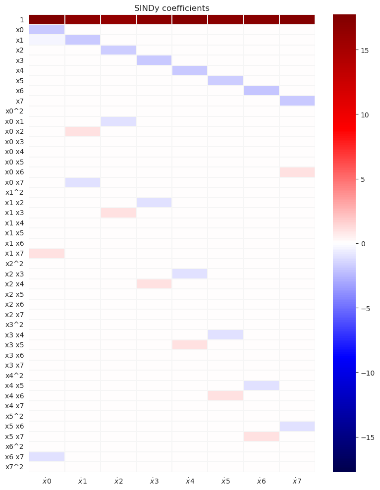
axs.set(title="SINDy coefficients")
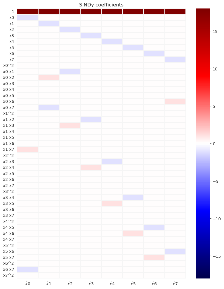
We can see that the SINDy model captures correctly the dominant terms and gives quite accurate predictions for the model coefficients and the value of the forcing. The subgrid forcing does not appear in this prediction.
Compare#
Same initial conditions#
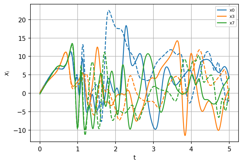
sindy_simulation = model.simulate(X_init, t=t)
fig, ax = plt.subplots(1, 1, figsize=(6, 4), dpi=150)
for i, component in enumerate(np.linspace(0, K - 1, num=3, dtype=int)):
    ax.plot(t, X[:, component], "--", color=colors[i])
    ax.plot(
        t,
        sindy_simulation[:, component],
        color=colors[i],
        label=model.feature_names[component],
    )
ax.legend(fontsize=7)
ax.set(xlabel="t", ylabel=r"$x_i$")
ax.grid()
plt.show();
Other initial conditions#
X_init_new = 0.5 * s(k, K) * (s(k, K) - 2) * (s(k, K) + 2)
W.set_state(X_init_new, Y_init)
# Run the true state
X_new, Y_new, t = W.run(dt, dt * steps, store=True)
sindy_simulation_new = model.simulate(X_init_new, t=t)
fig, ax = plt.subplots(1, 1, figsize=(6, 4), dpi=150)
for i, component in enumerate(np.linspace(0, K - 1, num=3, dtype=int)):
    ax.plot(t, X_new[:, component], "--", color=colors[i])
    ax.plot(
        t,
        sindy_simulation_new[:, component],
        color=colors[i],
        label=model.feature_names[component],
    )
ax.legend(fontsize=7)
ax.set(xlabel="t", ylabel=r"$x_i$", title="New initial conditions")
ax.grid()
plt.show();
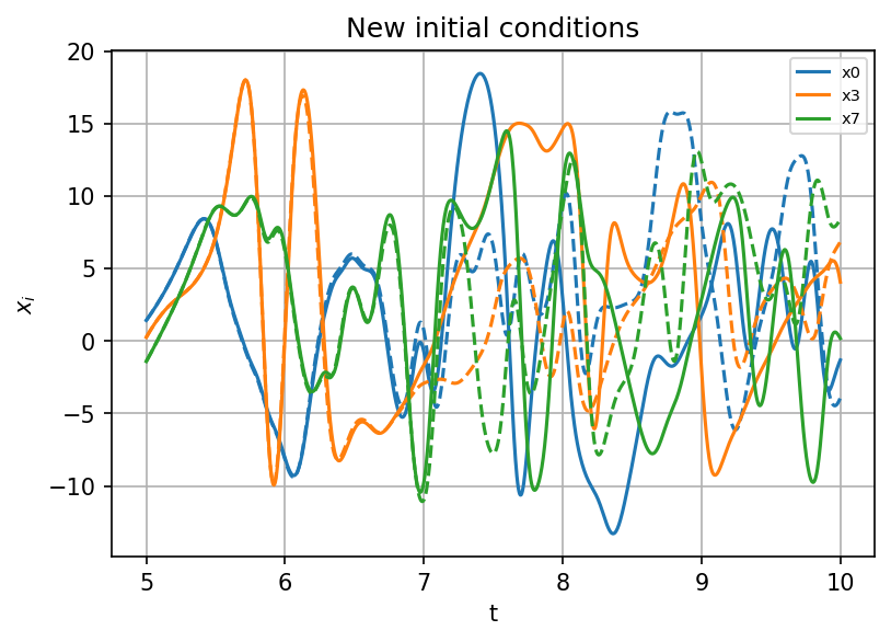
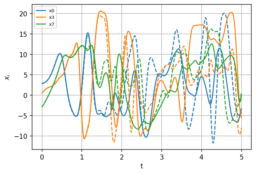
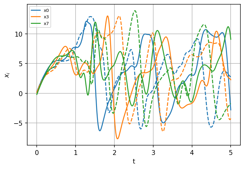
Similar to the case with L63 model, the system predicted by SINDy gives an accurate prediction of trajectories for a certain time, then the prediction strts deviating from the original model. It is related to the error in the coefficients obtained in optimization anf the chaotical nature of the Lorenz system.
X_init_new = s(k, K) * (s(k, K) - 2) * (s(k, K) + 2) # Initial conditions
X_new, t = integrate_L96_1t(X_init_new, Forcing, dt, steps)
sindy_simulation_new = model.simulate(X_init_new, t=t)
fig, ax = plt.subplots(1, 1, figsize=(6, 4), dpi=150)
for i, component in enumerate(np.linspace(0, K - 1, num=3, dtype=int)):
    ax.plot(t, X_new[:, component], "--", color=colors[i])
    ax.plot(
        t,
        sindy_simulation_new[:, component],
        color=colors[i],
        label=model.feature_names[component],
    )
ax.legend(fontsize=7)
ax.set(xlabel="t", ylabel=r"$x_i$")
ax.grid()
plt.show()
Case of strong coupling#
Now, let us consider the L96 two-scale model with a stronger coupling between the large and small scales. The coupling coefficient here is put to be 10 times higher.
# Create a "real world" with K=8 and J=32
W_strong = L96(K, J, F=Forcing, h=1.0)
W_strong.set_state(X_init, Y_init)
# Run the true state
X_s, Y_s, t = W_strong.run(dt, dt * steps, store=True)
fig, ax = plt.subplots(1, 1, figsize=(6, 4), dpi=150)
contours = ax.contourf(k, t, X_s, levels=20)
fig.colorbar(contours)
ax.set(xlabel="k", ylabel="t")
plt.show()
Build the SINDy model#
model_s = ps.SINDy(
    differentiation_method=differentiation_method,
    feature_library=feature_library,
    optimizer=optimizer,
    feature_names=[("x" + str(i)) for i in k],
)
model_s.fit(X_s, t=t)
SINDy(differentiation_method=SINDyDerivative(k=1, kind='finite_difference'),
      feature_library=PolynomialLibrary(),
      feature_names=['x0', 'x1', 'x2', 'x3', 'x4', 'x5', 'x6', 'x7'],
      optimizer=STLSQ(threshold=0.3))
In a Jupyter environment, please rerun this cell to show the HTML representation or trust the notebook. On GitHub, the HTML representation is unable to render, please try loading this page with nbviewer.org.
SINDy(differentiation_method=SINDyDerivative(k=1, kind='finite_difference'),
      feature_library=PolynomialLibrary(),
      feature_names=['x0', 'x1', 'x2', 'x3', 'x4', 'x5', 'x6', 'x7'],
optimizer=STLSQ(threshold=0.3))PolynomialLibrary()
PolynomialLibrary()
STLSQ(threshold=0.3)
STLSQ(threshold=0.3)
model_s.print()
(x0)' = 17.721 1 + -1.812 x0 + -0.348 x1 + 1.053 x1 x7 + -1.019 x6 x7
(x1)' = 16.639 1 + -1.877 x1 + 1.008 x0 x2 + -0.994 x0 x7
(x2)' = 16.293 1 + -1.746 x2 + -1.010 x0 x1 + 1.010 x1 x3
(x3)' = 16.817 1 + -1.801 x3 + -1.009 x1 x2 + 1.002 x2 x4
(x4)' = 17.244 1 + -1.874 x4 + -1.016 x2 x3 + 1.018 x3 x5
(x5)' = 16.967 1 + -1.785 x5 + -1.004 x3 x4 + 1.002 x4 x6
(x6)' = 17.114 1 + -1.946 x6 + -1.011 x4 x5 + 1.022 x5 x7
(x7)' = 17.387 1 + -1.808 x7 + 0.991 x0 x6 + -1.004 x5 x6
with sns.axes_style(style="white", rc={"axes.facecolor": (0, 0, 0, 0)}):
    max_mag = np.max(np.abs(model_s.coefficients()))
    fig, axs = plt.subplots(
        1, 1, figsize=(8, 10), sharey=True, sharex=True, tight_layout=True
    )
    plot_coefficients(
        model_s.coefficients(),
        input_features=[("x" + str(i)) for i in k],
        feature_names=feature_library.get_feature_names(),
        ax=axs,
        cbar=True,
        vmax=max_mag,
        vmin=-max_mag,
        cmap="seismic",
    )
    axs.set(title="SINDy coefficients")
We can see that despite the fact that in general SINDy captures the structure of ODEs, the coefficients become different from the original model, due to the influence of the interaction with the small scale. Interestingly, the coefficients in front of linear terms in the ODEs are now all close to 1.7-1.8 (instead of 1.0 in the true model), and the predicted forcing value is systematically smaller than the true value 18.
Run the predicted model#
sindy_simulation_s = model_s.simulate(X_init, t=t)
fig, ax = plt.subplots(1, 1, figsize=(6, 4), dpi=150)
for i, component in enumerate(np.linspace(0, K - 1, num=3, dtype=int)):
    ax.plot(t, X_s[:, component], "--", color=colors[i])
    ax.plot(
        t,
        sindy_simulation_s[:, component],
        color=colors[i],
        label=model.feature_names[component],
    )
ax.legend(fontsize=7)
ax.set(xlabel="t", ylabel=r"$x_i$")
ax.grid()
plt.show()
The resulting trajectories start deviating fast from the true trajectories.
Conclusions#
Sparse system identification method works well in conditions when we have already have some knowledgement about the equations (about sparsity, the type on non-lineartity) and optimal data representation (good coordinates).