Symbolic Regression vs. Neural Networks on Multiscale L96#
To recap from the previous notebooks, Lorenz (1996) describes a “two time-scale” model in two equations which are:
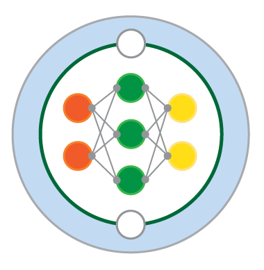
This model can be visualized as follows:

Fig. 8 Visualisation of a two-scale Lorenz ‘96 system with J = 8 and K = 6. Global-scale variables (\(X_k\)) are updated based on neighbouring variables and on the local-scale variables (\(Y_{j,k}\)) associated with the corresponding global-scale variable. Local-scale variabless are updated based on neighbouring variables and the associated global-scale variable. The neighbourhood topology of both local and global-scale variables is circular. Image from Exploiting the chaotic behaviour of atmospheric models with reconfigurable architectures - Scientific Figure on ResearchGate..#
import os
import time
from IPython.display import display, SVG

import gplearn
import gplearn.genetic
import matplotlib.pyplot as plt
import numpy as np
import pandas as pd
import pydot
import pysindy as ps
import torch
import torch.nn.functional as F
from sklearn.linear_model import LinearRegression
from sklearn.metrics import r2_score
from sklearn.preprocessing import PolynomialFeatures
from torch import nn, optim
from torch.utils.data import DataLoader, TensorDataset

from L96_model import L96
# Ensuring reproducibility
np.random.seed(14)
torch.manual_seed(14);
Dataset Generation#
Let’s generate some data using the same conditions as in the previous notebooks Introduction to Neural Networks and Using Neural Networks for L96 Parameterization.
Obtaining the Ground Truth#
time_steps = 20000
forcing, dt, T = 18, 0.01, 0.01 * time_steps

W = L96(8, 32, F=forcing)

X_true, _, _, subgrid_tend = W.run(dt, T, store=True, return_coupling=True)
X_true, subgrid_tend = X_true.astype(np.float32), subgrid_tend.astype(np.float32)

print(f"X_true shape: {X_true.shape}")
print(f"subgrid_tend shape: {subgrid_tend.shape}")
X_true shape: (20001, 8)
subgrid_tend shape: (20001, 8)
In this case, although we have 8 different dimensions in \(X\), each is derived in the exact same way from neighboring values of \(X\) (and local subdimensions \(Y\)). Therefore, we can actually reduce this problem from an 8-to-8D regression problem down to an 8-to-1D regression problem:
Dx = X_true.shape[1]
inputs = np.vstack([X_true[:, range(-i, Dx - i)] for i in range(Dx)])
targets = np.hstack([subgrid_tend[:, -i] for i in range(Dx)])

print(f"inputs shape: {inputs.shape}")
print(f"targets shape: {targets.shape}")
inputs shape: (160008, 8)
targets shape: (160008,)
Show code cell source
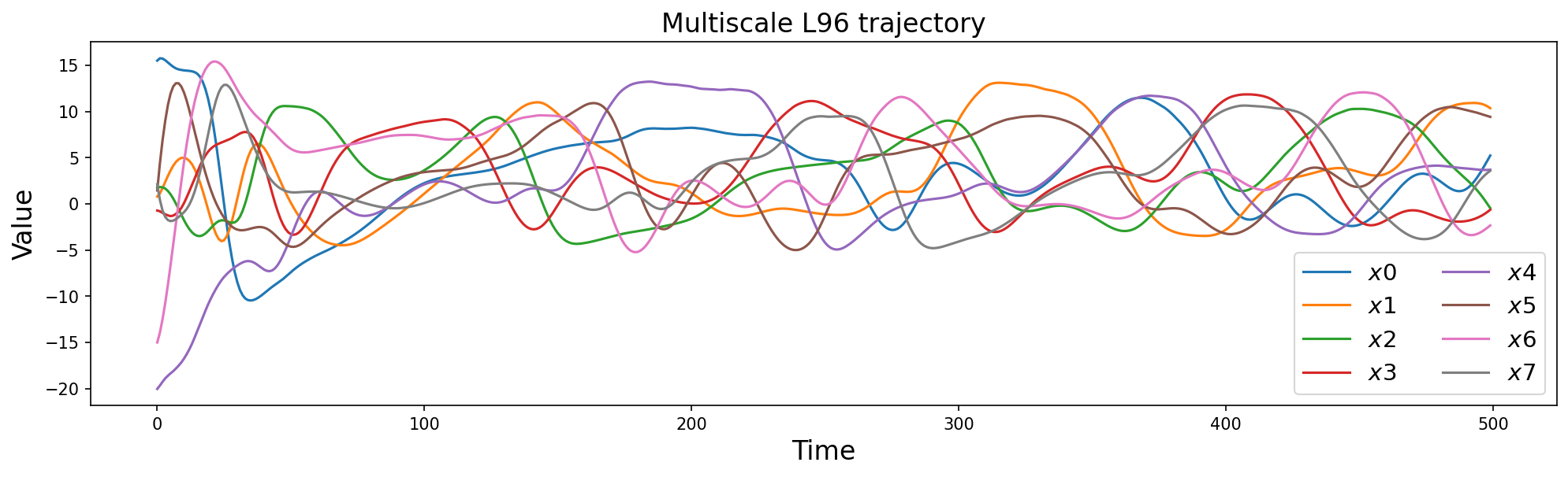
plt.figure(figsize=(16, 4), dpi=150)
plt.title("Multiscale L96 trajectory", fontsize=16)
for i in range(Dx):
    plt.plot(inputs[:, i][:500], label=r"$x" + str(i) + "$")
plt.legend(ncol=2, fontsize=14)
plt.xlabel("Time", fontsize=16)
plt.ylabel("Value", fontsize=16)
plt.show()
Show code cell source
fig = plt.figure(figsize=(12, 6), dpi=150)
fig.suptitle("2D histograms of features vs. forcing", fontsize=16)
for i in range(Dx):
    plt.subplot(2, 4, i + 1)
    plt.hist2d(inputs[:, i], targets, bins=50)
    plt.xlabel(f"$x_{i}$", fontsize=16)
    plt.xticks(np.arange(-6, 13, 2))
    plt.xlim(-8, 14)
    if i % 4 == 0:
        plt.ylabel("Forcing", fontsize=16)
plt.tight_layout()
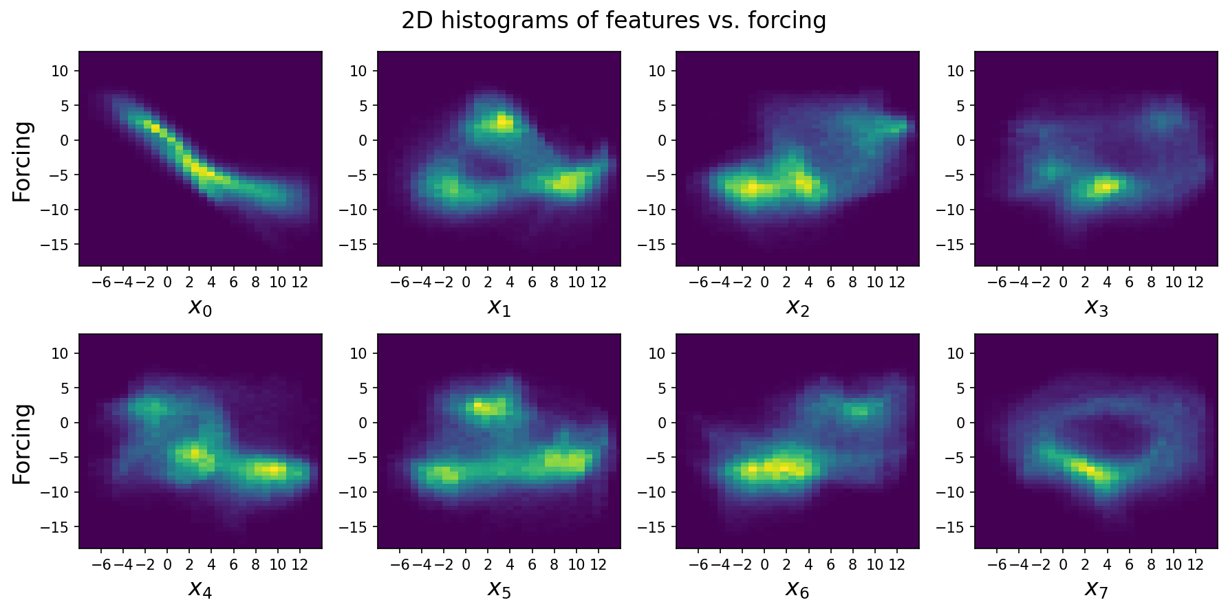
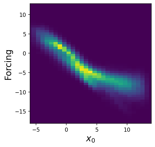
Looking at these marginal histograms of each large-scale variable vs. the subgrid forcing, we can see there’s a mostly linear relationship between \(x_0\) and its forcing, suggesting that the subgrid terms tend to force small values higher and large values lower. This suggests that an extremely simple linear model only containing \(x_0\) with negative slope will do reasonably well. However, the relationship isn’t completely linear, and also contains a bifurcation at larger \(x_0\).
For the other features, the relationships are less straightforward, but there’s clearly high mutual information.
Split the Data into Training and Test Sets#
data_idxs = np.arange(len(inputs))
np.random.shuffle(data_idxs)

num_train_samples = int(len(inputs) * 0.75)
train_idxs = data_idxs[:num_train_samples]
test_idxs = data_idxs[num_train_samples:]
Build the Dataset and the Dataloaders#
BATCH_SIZE = 1024

# Training Data
train_dataset = TensorDataset(
    torch.tensor(inputs[train_idxs]), torch.tensor(targets[train_idxs])
)
loader_train = DataLoader(dataset=train_dataset, batch_size=BATCH_SIZE, shuffle=True)

# Test Data
test_dataset = TensorDataset(
    torch.tensor(inputs[test_idxs]), torch.tensor(targets[test_idxs])
)
loader_test = DataLoader(dataset=test_dataset, batch_size=BATCH_SIZE, shuffle=True)
Creating and Training the Neural Network#
Now let’s create a neural network and train it on the dataset we generated above.
Define Functions to Train and Evaluate the Model#
Note
The code in this section is taken from the notebook Introduction to Neural Networks.
Show code cell content
def train_model(network, criterion, loader, optimizer):
    """Train the network for one epoch"""
    network.train()

    train_loss = 0
    for batch_x, batch_y in loader:
        # Get predictions
        if len(batch_x.shape) == 1:
            # This if block is needed to add a dummy dimension if our inputs are 1D
            # (where each number is a different sample)
            prediction = torch.squeeze(network(torch.unsqueeze(batch_x, 1)))
        else:
            prediction = network(batch_x)

        # Compute the loss
        loss = criterion(prediction, batch_y)
        train_loss += loss.item()

        # Clear the gradients
        optimizer.zero_grad()

        # Backpropagation to compute the gradients and update the weights
        loss.backward()
        optimizer.step()

    return train_loss / len(loader)


def test_model(network, criterion, loader):
    """Test the network"""
    network.eval()  # Evaluation mode (important when having dropout layers)

    test_loss = 0
    with torch.no_grad():
        for batch_x, batch_y in loader:
            # Get predictions
            if len(batch_x.shape) == 1:
                # This if block is needed to add a dummy dimension if our inputs are 1D
                # (where each number is a different sample)
                prediction = torch.squeeze(network(torch.unsqueeze(batch_x, 1)))
            else:
                prediction = network(batch_x)

            # Compute the loss
            loss = criterion(prediction, batch_y)
            test_loss += loss.item()

        # Get an average loss for the entire dataset
        test_loss /= len(loader)

    return test_loss


def fit_model(network, criterion, optimizer, train_loader, val_loader, n_epochs):
    """Train and validate the network"""
    train_losses, val_losses = [], []
    start_time = time.time()
    for epoch in range(1, n_epochs + 1):
        train_loss = train_model(network, criterion, train_loader, optimizer)
        val_loss = test_model(network, criterion, val_loader)
        train_losses.append(train_loss)
        val_losses.append(val_loss)
    end_time = time.time()
    print(f"Training completed in {int(end_time - start_time)} seconds.")

    return train_losses, val_losses
Create the Neural Network#
class Net_ANN(nn.Module):
    def __init__(self):
        super(Net_ANN, self).__init__()
        self.linear1 = nn.Linear(8, 16)
        self.linear2 = nn.Linear(16, 16)
        self.linear3 = nn.Linear(16, 1)

    def forward(self, x):
        x = F.relu(self.linear1(x))
        x = F.relu(self.linear2(x))
        x = self.linear3(x)[:, 0]
        return x
Train the Network#
nn_3l = Net_ANN()

n_epochs = 20
criterion = torch.nn.MSELoss()
optimizer = optim.Adam(nn_3l.parameters(), lr=0.01)
train_loss, validation_loss = fit_model(
    nn_3l, criterion, optimizer, loader_train, loader_test, n_epochs
)
Training completed in 17 seconds.
Visualize Results#
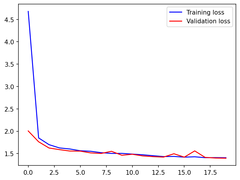
plt.figure(dpi=150)
plt.plot(train_loss, "b", label="Training loss")
plt.plot(validation_loss, "r", label="Validation loss")
plt.legend();
preds_nn = nn_3l(torch.from_numpy(inputs[test_idxs])).detach().numpy()
print("R2 Score:", r2_score(preds_nn, targets[test_idxs]))
R2 Score: 0.9223949649031744
The neural network gets an \(R^2\) of ~ 0.916, which seems pretty good given the non-determinism of the problem.
Comparing with Linear Regression#
linear_reg = LinearRegression()
linear_reg.fit(inputs[train_idxs], targets[train_idxs])
print("R2 Score:", linear_reg.score(inputs[test_idxs], targets[test_idxs]))
R2 Score: 0.8160184487760795
Linear regression also does fairly well, though about 0.1 lower in terms of \(R^2\). Lets look at its coefficients:
plt.figure(dpi=150)
plt.bar(range(8), linear_reg.coef_)
plt.xticks(range(8), [f"x{i}" for i in range(8)], fontsize=12)
plt.ylabel("Coefficient value", fontsize=12)
plt.show()
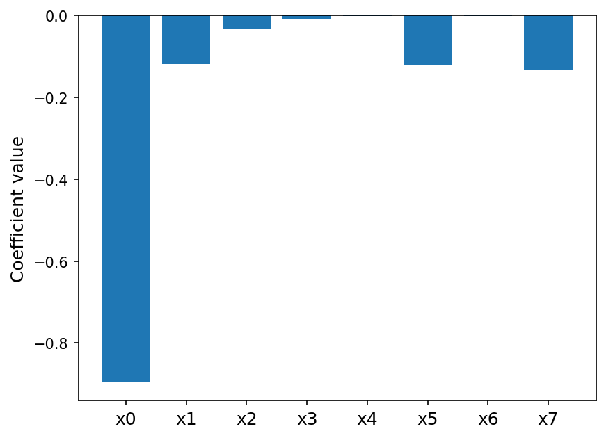
This matches the 2D histogram plots from earlier that showed a negative linear relationship between forcing and \(x_0\).
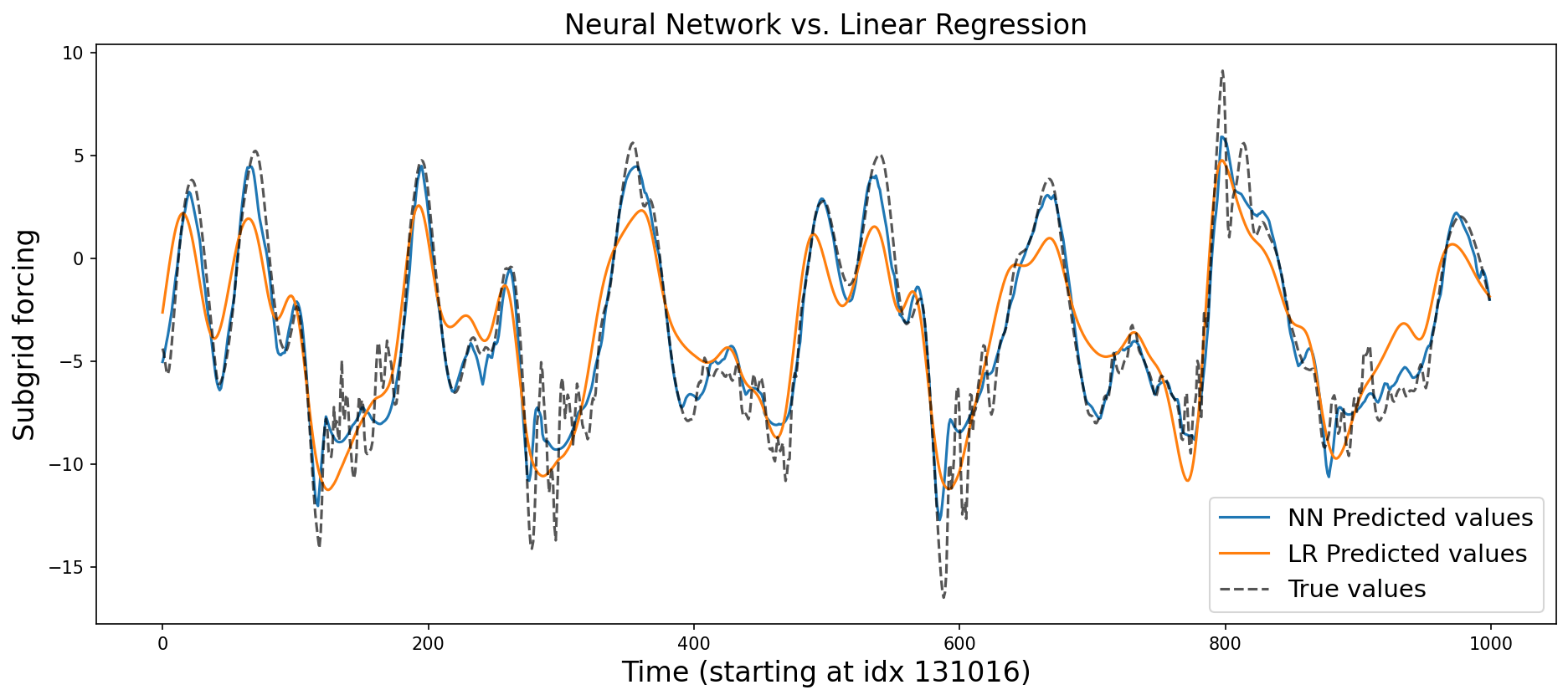
plt.figure(figsize=(15, 6), dpi=150)
plt.title("Neural Network vs. Linear Regression", fontsize=16)

preds_nn = nn_3l(torch.from_numpy(inputs)).detach().numpy()
preds_lr = linear_reg.predict(inputs)
random_idx = np.random.choice(len(targets - 1000))
random_slice = slice(random_idx, random_idx + 1000)

plt.plot(preds_nn[random_slice], label="NN Predicted values")
plt.plot(preds_lr[random_slice], label="LR Predicted values")
plt.plot(
    targets[random_slice], label="True values", ls="--", color="black", alpha=0.667
)
plt.xlabel(f"Time (starting at idx {random_idx})", fontsize=16)
plt.ylabel("Subgrid forcing", fontsize=16)
plt.legend(fontsize=14)
plt.show()
Symbolic regression with genetic programming#
Let’s try using one of the genetic programming libraries to discover a parameterization:
symbolic_reg = gplearn.genetic.SymbolicRegressor(
    population_size=5000,
    generations=25,
    p_crossover=0.7,
    p_subtree_mutation=0.1,
    p_hoist_mutation=0.05,
    p_point_mutation=0.1,
    max_samples=0.9,
    verbose=1,
    parsimony_coefficient=0.001,
    const_range=(-2, 2),
    function_set=("add", "mul", "sub", "div", "sin", "log"),
)

symbolic_reg.fit(inputs[train_idxs][:20000], targets[train_idxs][:20000])
    |   Population Average    |             Best Individual              |
---- ------------------------- ------------------------------------------ ----------
 Gen   Length          Fitness   Length          Fitness      OOB Fitness  Time Left
   0    15.09          2250.77        3          1.64883          1.66775      3.21m
   1    10.32          6.53204        5          1.62545          1.63651      3.13m
   2    12.32          16.9512        5          1.62268          1.66148      3.04m
   3     7.04          5.26195       20          1.57546           1.6044      2.26m
   4     5.07          9.58891       24          1.55363          1.55098      1.84m
   5     5.79          5.96614       21          1.51949          1.49863      1.97m
   6     9.63          4.65507       17          1.50515          1.50598      2.64m
   7    16.11          2.78142       28          1.47296          1.45776      3.67m
   8    19.77          2.69051       28           1.4555          1.46709      3.93m
   9    21.42          2.80303       41          1.45297          1.48639      3.84m
  10    22.63          2.61995       37          1.44204          1.47566      3.98m
  11    23.78          2.29202       41          1.42739           1.4853      3.87m
  12    24.47           6.6118        8          1.41676          1.43687      3.60m
  13    25.15          2.55741       22           1.4201          1.47976      3.29m
  14    25.67          2.27797       28          1.41595          1.43681      2.97m
  15    24.77          2.45272       42          1.35228          1.38372      2.61m
  16    20.61          3.97112       23          1.34902          1.34875      2.02m
  17    12.16          3.66793       24          1.33076          1.35901      1.30m
  18    14.17          3.62681       24          1.32406          1.35392      1.30m
  19    27.37          2.86559       29          1.31132          1.33767      1.82m
  20    25.82          2.40423       31          1.30332          1.33496      1.41m
  21    23.41          2.45246       38          1.30026          1.32775     59.04s
  22    23.45          2.57487       38          1.29615          1.31448     38.19s
  23    24.97          2.56582       33          1.29189          1.30837     19.99s
  24    24.11          2.33584       37          1.29417          1.32678      0.00s
sub(sin(mul(-0.447, X0)), sub(X0, sin(sub(-1.107, log(add(X2, sub(sub(sub(-1.107, log(add(X2, sub(sin(sub(-1.107, log(mul(-0.447, X0)))), sub(X0, -0.220))))), X0), log(sin(mul(-0.447, X0))))))))))In a Jupyter environment, please rerun this cell to show the HTML representation or trust the notebook.
On GitHub, the HTML representation is unable to render, please try loading this page with nbviewer.org.
sub(sin(mul(-0.447, X0)), sub(X0, sin(sub(-1.107, log(add(X2, sub(sub(sub(-1.107, log(add(X2, sub(sin(sub(-1.107, log(mul(-0.447, X0)))), sub(X0, -0.220))))), X0), log(sin(mul(-0.447, X0))))))))))
print(symbolic_reg._program)
sub(sin(mul(-0.447, X0)), sub(X0, sin(sub(-1.107, log(add(X2, sub(sub(sub(-1.107, log(add(X2, sub(sin(sub(-1.107, log(mul(-0.447, X0)))), sub(X0, -0.220))))), X0), log(sin(mul(-0.447, X0))))))))))
print(
    "R2 Score:", r2_score(symbolic_reg.predict(inputs[test_idxs]), targets[test_idxs])
)
R2 Score: 0.8499308040527297
While the program does slightly better than linear regression, it’s extremely complicated (graph visualization below for slightly easier inspection):
# Build the graph
graph = pydot.graph_from_dot_data(symbolic_reg._program.export_graphviz())[0]
graph.write_svg("figs/symbolic_regression.svg")

# Display the graph
display(SVG("figs/symbolic_regression.svg"))

Explore the Pareto frontier#
We can explore the Pareto frontier of the final population of programs as well, to see if there’s a simpler program that still does well
df = pd.DataFrame.from_dict(
    [
        dict(
            idx=i,
            expr=str(p),
            fitness=p.fitness_,
            length=p.length_,
            r2_score=r2_score(p.execute(inputs[test_idxs]), targets[test_idxs]),
        )
        for i, p in enumerate(symbolic_reg._programs[-1])
    ]
)
pareto_frontier = []
used_programs = set()

for l in range(1, 40):
    programs = df[df.length <= l]
    best = programs.r2_score.argmax()
    idx = programs.idx.values[best]
    r2 = programs.r2_score.values[best]
    program = symbolic_reg._programs[-1][idx]
    if program not in used_programs:
        pareto_frontier.append(dict(length=l, r2=r2, expr=str(program)))
        used_programs.add(program)

pd.set_option("max_colwidth", 200)
pareto_frontier = pd.DataFrame.from_dict(pareto_frontier)
pareto_frontier
| length | r2 | expr | |
|---|---|---|---|
| 0 | 1 | 0.000000 | -0.220 |
| 1 | 2 | 0.000000 | sin(-1.107) |
| 2 | 3 | 0.787718 | sub(-0.220, X0) |
| 3 | 8 | 0.837378 | sub(sin(mul(-0.447, X0)), sub(X0, -0.220)) |
| 4 | 11 | 0.841150 | sub(sin(mul(-0.447, X0)), sub(X0, sin(mul(-0.447, X0)))) |
| 5 | 12 | 0.842545 | sub(sin(sin(mul(-0.447, X0))), sub(X0, sin(mul(-0.447, X0)))) |
| 6 | 13 | 0.843272 | sub(sin(sin(mul(-0.447, X0))), sub(X0, sin(sin(mul(-0.447, X0))))) |
| 7 | 16 | 0.854240 | sub(sin(mul(-0.447, X0)), sub(X0, sin(sub(-1.107, log(add(X2, div(X0, -1.107))))))) |
| 8 | 17 | 0.855131 | sub(sin(sub(-1.107, log(add(X2, sub(sin(X0), X0))))), sub(X0, sin(mul(-0.447, X0)))) |
| 9 | 19 | 0.856080 | sub(sin(sub(-1.107, log(add(X2, sub(sub(sin(X0), X0), -1.107))))), sub(X0, sin(mul(-0.447, X0)))) |
| 10 | 21 | 0.856531 | sub(sin(sub(-1.107, log(add(X2, sub(sub(-0.447, X0), log(sub(X0, -0.220))))))), sub(X0, sin(mul(-0.307, X0)))) |
| 11 | 23 | 0.856728 | sub(sin(sub(-1.107, log(add(X2, sub(sub(sin(X0), X0), log(sin(mul(-0.447, X0)))))))), sub(X0, sin(mul(-0.447, X0)))) |
| 12 | 35 | 0.856754 | sub(sin(sub(-1.107, log(add(X2, sub(sin(sub(-1.107, log(add(X2, sub(sub(sin(-0.605), X0), log(sub(X0, -0.220))))))), sub(X0, sin(mul(-0.447, X0)))))))), sub(X0, sin(mul(-0.447, X0)))) |
| 13 | 39 | 0.857035 | sub(sin(mul(-0.447, X0)), sub(X0, sin(sub(-1.107, log(add(X2, sub(sub(sin(sub(-1.107, log(add(X2, sub(sub(-0.605, X0), log(sub(-0.447, X0))))))), sub(X0, sin(mul(-0.447, X0)))), log(mul(-0.447, X0... |
Unfortunately, nothing really jumps out here as both simple and performant.
Symbolic Regression with Sparse Linear Regression and Polynomial Features#
We can also apply sparse regression methods to this problem with polynomial features
def learned_expr(coef, names, cutoff=1e-3):
    coef_idx = np.argwhere(np.abs(coef) > cutoff)[:, 0]
    sort_order = reversed(np.argsort(np.abs(coef[coef_idx])))
    return " + ".join(
        [
            f"{coef[coef_idx[i]]:.4f}*{names[coef_idx[i]].replace(' ','*')}"
            for i in sort_order
        ]
    )
pf = PolynomialFeatures(2)
feats = pf.fit_transform(inputs)
names = pf.get_feature_names_out([f"x_{i}" for i in range(8)])
Non-sparse linear regression#
linear_reg = LinearRegression()
linear_reg.fit(feats[train_idxs], targets[train_idxs])
learned_expr(linear_reg.coef_, names)
'-0.6913*x_0 + 0.4333*x_1 + 0.3393*x_7 + 0.2112*x_5 + 0.1420*x_6 + 0.1118*x_2 + -0.0399*x_0*x_1 + -0.0333*x_0*x_2 + -0.0323*x_6*x_7 + -0.0288*x_0*x_7 + -0.0283*x_1*x_2 + -0.0248*x_1*x_5 + -0.0242*x_3 + -0.0219*x_1*x_6 + -0.0209*x_5*x_7 + 0.0201*x_0^2 + -0.0185*x_1*x_4 + -0.0135*x_0*x_5 + 0.0124*x_0*x_3 + 0.0107*x_4 + 0.0099*x_1*x_3 + 0.0090*x_2*x_5 + -0.0088*x_4*x_7 + -0.0081*x_5^2 + -0.0076*x_2*x_3 + -0.0074*x_2*x_7 + 0.0071*x_3*x_4 + 0.0071*x_4*x_5 + -0.0069*x_3*x_5 + 0.0061*x_3*x_6 + 0.0059*x_1*x_7 + -0.0057*x_7^2 + 0.0050*x_3^2 + -0.0048*x_0*x_4 + -0.0045*x_1^2 + -0.0036*x_0*x_6 + -0.0036*x_3*x_7 + 0.0034*x_2^2 + 0.0024*x_4*x_6 + 0.0023*x_2*x_4 + 0.0015*x_2*x_6 + -0.0011*x_5*x_6'
print("R2 Score:", linear_reg.score(feats[test_idxs], targets[test_idxs]))
R2 Score: 0.8872654640415502
Adding polynomial features brings our \(R^2\) much closer to that of the neural network, but we have a ton of terms. Let’s try making the regression sparser.
Sequentially thresholded least squares#
stlsq = ps.optimizers.stlsq.STLSQ(alpha=0.001, threshold=0.01)
stlsq.fit(feats[train_idxs], targets[train_idxs])
learned_expr(stlsq.coef_[0], names)
'-3.7208*1 + -0.7842*x_0 + 0.3574*x_1 + 0.2431*x_7 + 0.1900*x_2 + 0.1778*x_5 + 0.1522*x_6 + -0.0390*x_0*x_1 + -0.0356*x_0*x_2 + -0.0335*x_6*x_7 + 0.0267*x_0^2 + -0.0265*x_1*x_5 + -0.0257*x_0*x_7 + -0.0227*x_1*x_2 + 0.0189*x_4 + -0.0164*x_1*x_6 + -0.0156*x_5*x_7 + 0.0145*x_3 + -0.0120*x_0*x_5 + 0.0110*x_0*x_3'
stlsq.score(feats[test_idxs], targets[test_idxs])
0.882294259449451
Looks like we can get a much sparser expression without sacrificing too much performance, though if we increase the threshold slightly, we will see a trade-off:
stlsq2 = ps.optimizers.stlsq.STLSQ(alpha=0.001, threshold=0.02)
stlsq2.fit(feats[train_idxs], targets[train_idxs])
learned_expr(stlsq2.coef_[0], names)
'-1.5860*1 + -0.9857*x_0 + 0.1324*x_2 + 0.0728*x_3 + -0.0725*x_7 + -0.0436*x_1 + -0.0322*x_0*x_2 + 0.0307*x_0^2'
stlsq2.score(feats[test_idxs], targets[test_idxs])
0.861645175881121
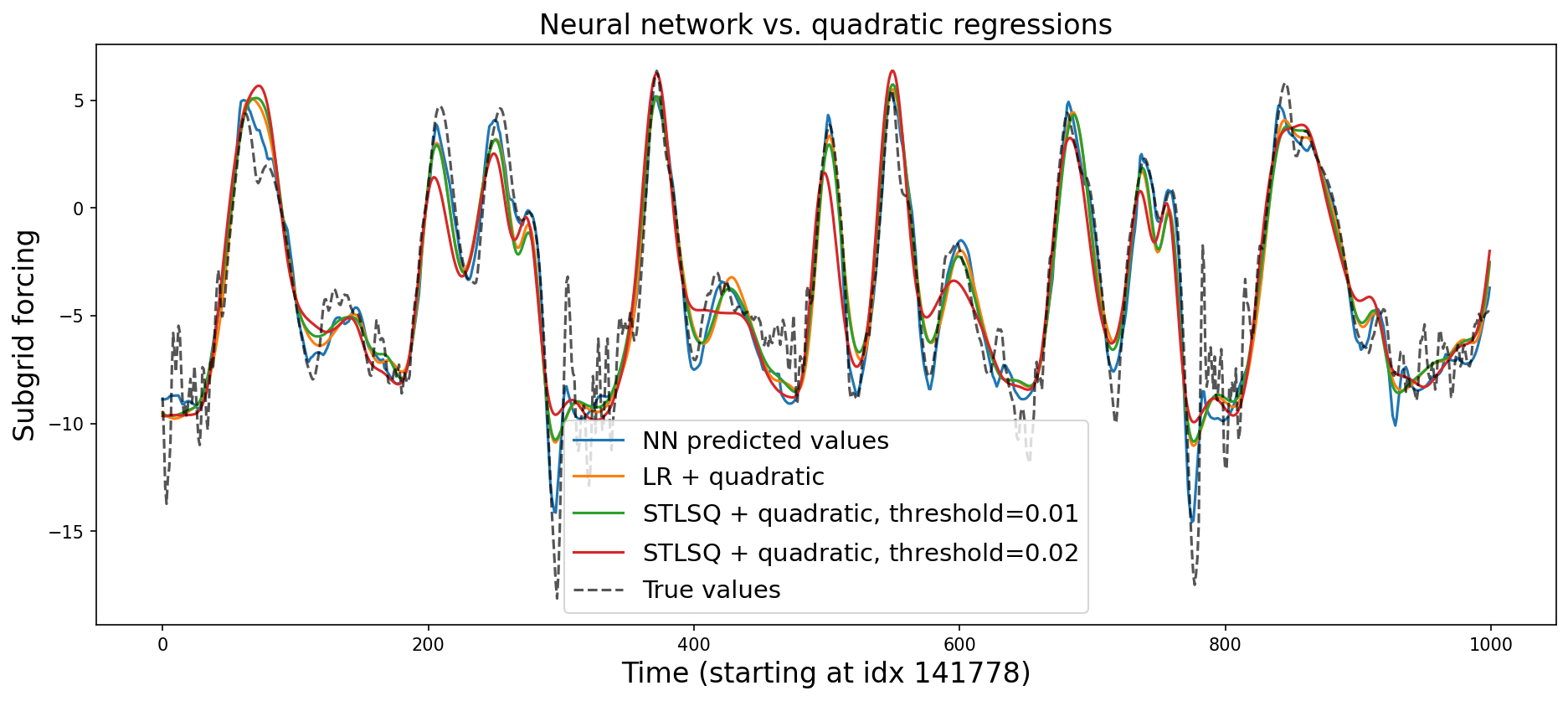
This is much simpler, but less performant. It still strongly outperformed the particluar genetic programming method we used, though. Let’s visualize some of the predictions:
plt.figure(figsize=(15, 6), dpi=150)
plt.title("Neural network vs. quadratic regressions", fontsize=16)

preds_nn = nn_3l(torch.from_numpy(inputs)).detach().numpy()
preds_lr_quad = linear_reg.predict(feats)
preds_st_quad = stlsq.predict(feats)
preds_st_quad2 = stlsq2.predict(feats)
random_idx = np.random.choice(len(targets - 1000))
random_slice = slice(random_idx, random_idx + 1000)

plt.plot(preds_nn[random_slice], label="NN predicted values")
plt.plot(preds_lr_quad[random_slice], label="LR + quadratic")
plt.plot(preds_st_quad[random_slice], label=r"STLSQ + quadratic, threshold=$0.01$")
plt.plot(preds_st_quad2[random_slice], label=r"STLSQ + quadratic, threshold=$0.02$")
plt.plot(
    targets[random_slice], label="True values", ls="--", color="black", alpha=0.667
)
plt.xlabel(f"Time (starting at idx {random_idx})", fontsize=16)
plt.ylabel("Subgrid forcing", fontsize=16)
plt.legend(fontsize=14)
plt.show()
Add threshold features#
The 2D histogram of \(x_0\) looks like it might be potentially modelable by piecewise linear regression:
plt.figure(figsize=(4, 4), dpi=150)
plt.hist2d(inputs[:, 0], targets, bins=50)
plt.xlim(-6, 14)
plt.xlabel("$x_0$", fontsize=16)
plt.ylabel("Forcing", fontsize=16)
plt.show()
Sparse regression#
Let’s see if sparse regression will discover that if we provide it with thresholding features and cross-terms:
x0_thresholds = np.array(
    [np.ones_like(inputs[:, 0])] + [inputs[:, 0] > i for i in range(6)]
)
x0_threshold_names = [""] + [f"*(x0>{t})" for t in range(6)]

feats2 = np.array(
    [
        feats[:, i] * x0_thresholds[j]
        for i in range(feats.shape[1])
        for j in range(len(x0_thresholds))
    ]
).T
names2 = [
    f"{names[i]}{x0_threshold_names[j]}"
    for i in range(feats.shape[1])
    for j in range(len(x0_thresholds))
]
stlsq3 = ps.optimizers.stlsq.STLSQ(alpha=0.001, threshold=0.25)
stlsq3.fit(feats2[train_idxs], targets[train_idxs])
learned_expr(stlsq3.coef_[0], names2)
/usr/share/miniconda/envs/L96M2lines/lib/python3.9/site-packages/sklearn/utils/extmath.py:189: RuntimeWarning: invalid value encountered in matmul
  ret = a @ b
'-2.8051*1*(x0>4) + -0.9871*x_0 + -0.6571*1*(x0>2) + 0.6440*x_0*(x0>4) + -0.5681*1*(x0>0) + -0.5286*1*(x0>1) + -0.2734*1*(x0>5)'
stlsq3.score(feats2[test_idxs], targets[test_idxs])
0.8590951075317006
plt.figure(figsize=(4, 4), dpi=150)
plt.hist2d(inputs[:, 0], targets, bins=50)

fn = (
    lambda x0: -2.1200 * 1 * (x0 > 2)
    + -1.2695 * 1 * (x0 > 0)
    + -0.9488 * x0
    + -0.6694 * 1 * (x0 > 4)
    + 0.5175 * x0 * (x0 > 1)
)

xt = np.linspace(-6, 14, 100)
yt = fn(xt)
plt.plot(xt, yt, color="red")
plt.xlim(-6, 14)
plt.xlabel("$x_0$", fontsize=16)
plt.ylabel("Forcing", fontsize=16)
plt.show()

It looks like the model learns a piecewise linear function in a single variable, even though we didn’t explicitly require it!
Genetic programming#
We can also try using genetic programming here, but with a different function set that removes some of the nonlinear operators we included before and replaces them with min and max, which allow for piecewise behavior:
symbolic_reg_pw = gplearn.genetic.SymbolicRegressor(
    population_size=5000,
    generations=50,
    p_crossover=0.7,
    p_subtree_mutation=0.1,
    p_hoist_mutation=0.05,
    p_point_mutation=0.1,
    max_samples=0.9,
    verbose=1,
    parsimony_coefficient=0.001,
    const_range=(-2, 2),
    function_set=("add", "mul", "max", "min"),
)
symbolic_reg_pw.fit(inputs[train_idxs][:20000], targets[train_idxs][:20000])
    |   Population Average    |             Best Individual              |
---- ------------------------- ------------------------------------------ ----------
 Gen   Length          Fitness   Length          Fitness      OOB Fitness  Time Left
   0    27.65      3.78741e+06        7          2.45249          2.54746      5.82m
   1     8.00          9.51443        5          1.85843          1.82615      4.05m
   2    10.82          7.30098        3           1.6483          1.63764      4.45m
   3     8.34          27.6089        3          1.64321          1.68342      4.14m
   4     4.92          26.8323       15          1.50401          1.50866      3.69m
   5     3.87          16.3644       15          1.44304          1.44976      3.60m
   6     6.13           148.18       11          1.40594          1.42375      3.78m
   7    12.76          15.4382       13          1.37424          1.38711      4.78m
   8    14.48          10.2082       13           1.3658          1.36791      4.99m
   9    15.67          12.0612       21          1.35567          1.37664      5.04m
  10    15.53          17917.1       23           1.3514          1.40418      4.85m
  11    15.51          7.61133       29          1.35019          1.38838      4.88m
  12    16.27          4.11042       19          1.34782          1.38404      4.84m
  13    15.22          12.9581       23          1.34734          1.38836      4.57m
  14    14.50          1540.79       17          1.34519          1.40768      4.33m
  15    13.97          5.27408       17          1.34517          1.40786      4.14m
  16    14.09          13.3842       17          1.34172          1.43891      4.13m
  17    14.21          3.51828       13          1.34363          1.37425      3.95m
  18    14.46          84.8708       19          1.34315          1.43713      3.80m
  19    14.50           8.1359       15          1.33915          1.37526      3.66m
  20    14.49          4.71403       15          1.33942          1.41217      3.55m
  21    14.12          4.65016       15          1.33662          1.39804      3.38m
  22    13.77          38.3175       19          1.33467          1.42346      3.31m
  23    13.67          9.76407       17          1.33539          1.41711      3.10m
  24    13.87          9.07149       15          1.33255          1.43467      3.00m
  25    14.14          114.952       15          1.33405          1.42116      2.88m
  26    14.53          110.894       15          1.33412          1.42058      2.78m
  27    14.70          3.25037       19          1.33509          1.41981      2.68m
  28    14.72          10.7036       13          1.33059          1.37007      2.62m
  29    14.88          3.91762       25          1.32809          1.37427      2.45m
  30    14.62          6.29094       15          1.32687          1.39063      2.30m
  31    14.57           3.5343       17           1.3249          1.40442      2.18m
  32    14.12          3.90761       21          1.32425          1.41418      2.05m
  33    13.83          5.69476       13          1.32439          1.42588      1.97m
  34    13.48          8.32606       15          1.32568          1.40132      1.78m
  35    13.25          79.5995       17          1.32476          1.40569      1.66m
  36    13.24          4.45101       13          1.32515          1.41905      1.55m
  37    13.04          7.14949       13          1.32524           1.4182      1.41m
  38    13.15          5.93211       15          1.32344          1.42146      1.31m
  39    13.15          9.69874       17          1.32478          1.40562      1.22m
  40    13.18          5.74077       13          1.32703          1.40212      1.07m
  41    12.99          9.94645       13          1.32421          1.42748     56.92s
  42    12.99          4.36878       13          1.32517          1.41883     49.86s
  43    13.12          12.7419       13          1.32593          1.41204     42.96s
  44    13.26          3.95264       13          1.32416          1.42798     35.94s
  45    13.06          13.1207       21          1.32404          1.42906     29.54s
  46    13.04          6.56359       13          1.32464          1.42364     21.41s
  47    13.19          6.23439       21          1.32029          1.34429     14.35s
  48    13.10          27.2948       21          1.32101          1.33781      7.18s
  49    13.26          5.91966       21          1.31816          1.36342      0.00s
add(max(min(mul(max(X0, -1.442), -0.938), X1), -1.937), mul(min(X0, add(max(X5, X3), max(X6, X4))), -0.720))In a Jupyter environment, please rerun this cell to show the HTML representation or trust the notebook.
On GitHub, the HTML representation is unable to render, please try loading this page with nbviewer.org.
add(max(min(mul(max(X0, -1.442), -0.938), X1), -1.937), mul(min(X0, add(max(X5, X3), max(X6, X4))), -0.720))
print(symbolic_reg_pw._program)
add(max(min(mul(max(X0, -1.442), -0.938), X1), -1.937), mul(min(X0, add(max(X5, X3), max(X6, X4))), -0.720))
print(
    "R2 Score:",
    r2_score(symbolic_reg_pw.predict(inputs[test_idxs]), targets[test_idxs]),
)
R2 Score: 0.8354791875984894
While this leads to slightly higher \(R^2\) than before, the model is still pretty complex:
# Build the graph
graph = pydot.graph_from_dot_data(symbolic_reg_pw._program.export_graphviz())[0]
graph.write_svg("figs/symbolic_regression_pw.svg")

# Display the graph
from IPython.display import Image, display

display(SVG("figs/symbolic_regression_pw.svg"))

Tuning the hyperparameters could help, but requires more compute.