Improving Performance of Neural Networks#
In this notebook, we will briefly introduce several techniques that are generally used to improve the accuracy of neural networks.
%matplotlib inline
import time

import matplotlib.pyplot as plt
import numpy as np
import torch
from torch import nn, optim
from torch.utils.data import TensorDataset, DataLoader

from L96_model import L96
# Ensuring reproducibility
np.random.seed(14)
torch.manual_seed(14);
Setting up the Dataset, Model, and the Training Code#
First, we setup all the necessary code that’s required to build the dataset, create our neural network and train the network on the dataset.
Note
The dataset, the neural network, and the training and evaluation functions that we use in this notebook are same as the one defined in Introduction to Machine Learning and Neural Networks and Using Neural Networks for L96 Parameterization.
Create the Dataset#
Show code cell content
# Generating the Ground Truth
# ---------------------------

time_steps = 2000
forcing, dt, T = 18, 0.01, 0.01 * time_steps

W = L96(8, 32, F=forcing)

X_true, _, _, xy_true = W.run(dt, T, store=True, return_coupling=True)
X_true, xy_true = X_true.astype(np.float32), xy_true.astype(np.float32)


# Splitting the into Training and Test Dataset
# --------------------------------------------

val_size = 400

# Training Data
X_true_train = X_true[:-val_size, :]
subgrid_tend_train = xy_true[:-val_size, :]

# Test Data
X_true_test = X_true[-val_size:, :]
subgrid_tend_test = xy_true[-val_size:, :]


# Building the Dataset and the Dataloaders
# ----------------------------------------

BATCH_SIZE = 1024

# Training Data
nlocal_data = TensorDataset(
    torch.from_numpy(X_true_train),
    torch.from_numpy(subgrid_tend_train),
)
loader_train = DataLoader(dataset=nlocal_data, batch_size=BATCH_SIZE, shuffle=True)


# Test Data
nlocal_data_test = TensorDataset(
    torch.from_numpy(X_true_test), torch.from_numpy(subgrid_tend_test)
)
loader_test = DataLoader(dataset=nlocal_data_test, batch_size=BATCH_SIZE, shuffle=True)
Create the Neural Network#
We build a 3 layer neural network consisting of two hidden layers and an output layer. Each hidden layer is followed by the ReLU activation function.
Show code cell content
class NetANN(nn.Module):
    def __init__(self):
        super().__init__()
        self.linear1 = nn.Linear(8, 16)  # 8 inputs
        self.linear2 = nn.Linear(16, 16)
        self.linear3 = nn.Linear(16, 8)  # 8 outputs

        self.relu = nn.ReLU()

    def forward(self, x):
        x = self.relu(self.linear1(x))
        x = self.relu(self.linear2(x))
        x = self.linear3(x)
        return x
Train and Evaluate the Network#
Show code cell content
def train_model(network, criterion, loader, optimizer):
    """Train the network for one epoch"""
    network.train()

    train_loss = 0
    for batch_x, batch_y in loader:
        # Get predictions
        if len(batch_x.shape) == 1:
            # This if block is needed to add a dummy dimension if our inputs are 1D
            # (where each number is a different sample)
            prediction = torch.squeeze(network(torch.unsqueeze(batch_x, 1)))
        else:
            prediction = network(batch_x)

        # Compute the loss
        loss = criterion(prediction, batch_y)
        train_loss += loss.item()

        # Clear the gradients
        optimizer.zero_grad()

        # Backpropagation to compute the gradients and update the weights
        loss.backward()
        optimizer.step()

    return train_loss / len(loader)


def test_model(network, criterion, loader):
    """Test the network"""
    network.eval()  # Evaluation mode (important when having dropout layers)

    test_loss = 0
    with torch.no_grad():
        for batch_x, batch_y in loader:
            # Get predictions
            if len(batch_x.shape) == 1:
                # This if block is needed to add a dummy dimension if our inputs are 1D
                # (where each number is a different sample)
                prediction = torch.squeeze(network(torch.unsqueeze(batch_x, 1)))
            else:
                prediction = network(batch_x)

            # Compute the loss
            loss = criterion(prediction, batch_y)
            test_loss += loss.item()

        # Get an average loss for the entire dataset
        test_loss /= len(loader)

    return test_loss


def fit_model(network, criterion, optimizer, train_loader, val_loader, n_epochs):
    """Train and validate the network"""
    train_losses, val_losses = [], []
    start_time = time.time()
    for epoch in range(1, n_epochs + 1):
        train_loss = train_model(network, criterion, train_loader, optimizer)
        val_loss = test_model(network, criterion, val_loader)
        train_losses.append(train_loss)
        val_losses.append(val_loss)
    end_time = time.time()
    print(f"Training completed in {int(end_time - start_time)} seconds.")

    return train_losses, val_losses
Regularization and Overfitting#
One of the most common issues that happen while training a neural network is when the model memorizes the training dataset. It causes the model to perform very accurately on the training set but shows very poor performance on the validation set. This phenomenon is termed overfitting. One of the ways to prevent overfitting is to add regularization to our model as described below.
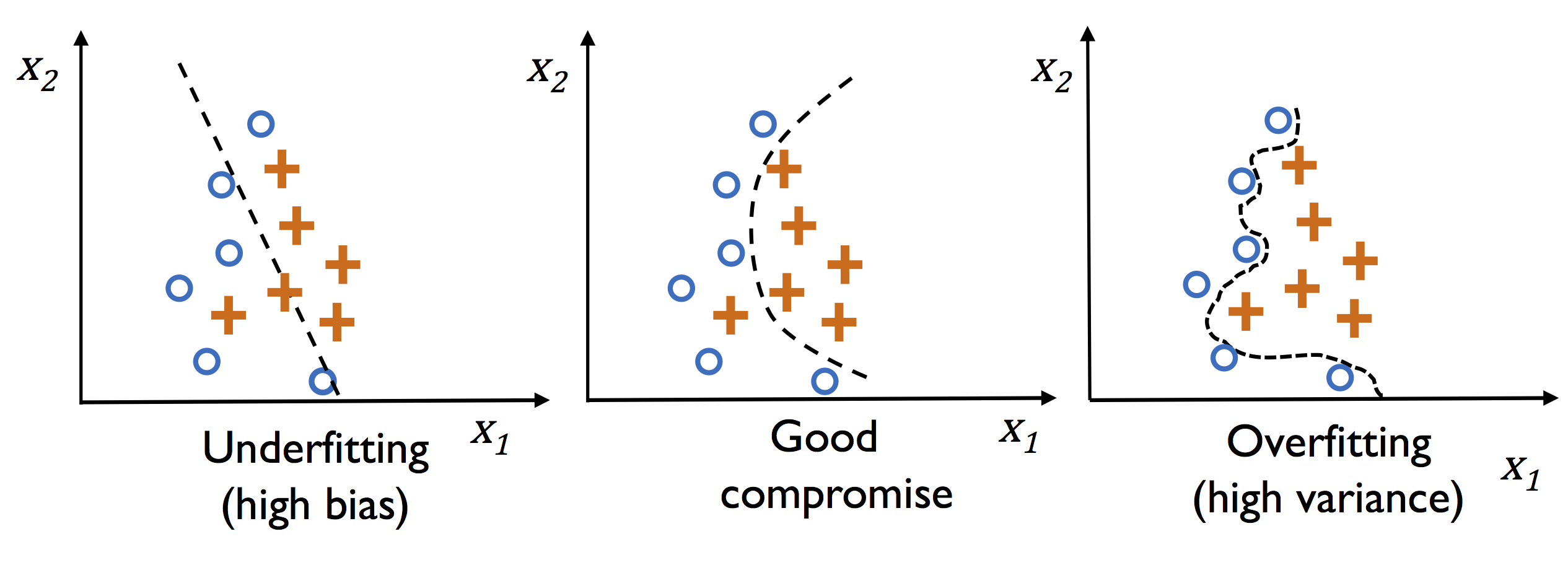
Fig. 3 Curves showing different types of model fits. The image is taken from the Python Machine Learning book by Sebastian Raschka.#
The curve on the far right of the plot above predicts perfectly on the given set, yet it’s not the best choice. This is because if you were to gather some new data points, they most likely would not be on that curve. Instead, those new points would be closer to the curve in the middle graph since it generalizes better to the dataset.
Regularization Intuition#
Regularization can be thought of as putting constraints on the model to obtain better generalizability i.e. avoiding remembering the training data.
One of the ways to achieve this can be by adding a term to the loss function such that:
Loss = Training Loss + Regularization
This puts a penalty for making the model more complex.
Very braodly speaking (just to gain intuition) - if we want to reduce the training loss (reduce bias) we should try using a more complex model (if we have enough data) and if we want to reduce overfitting (reduce variace) we should simplify or constraint the model (increase regularization).
Regularization of Neural Networks#
Some of the ways to add regularization in neural networks are:
Dropout (added in the definition of the network).
Early stopping
Weight decay (added in the optimizer part - see
optim.Adamin PyTorch)Data augmentation (usually for images)
Below we show how some of these regularizations can be applied to the L96 parameterization problem. However, this particular problem is not very plagued by the issue of overfitting, and so the advantages of these processes are not clear in all their glory.
Weight decay (L2 norm)#
Weight decay is usually defined as a term that’s added directly to the update rule. Namely, to update a certain weight \(w\) in the \(i+1\) iteration, we would use a modified rule:
\(w_{i+1} = w_{i} - \gamma ( \frac{\partial L}{\partial w} + A w_{i})\)
In practice, this is almost identical to L2 regularization, though there is some difference (e.g., see here)
Weight decay is one of the parameters of the optimizer - see torch.optim.SGD
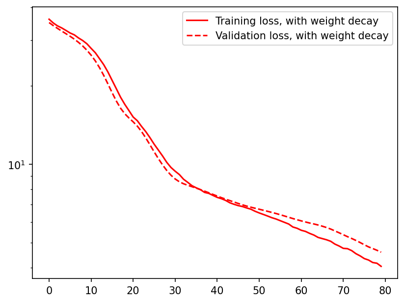
Using Weight Decay#
Now we try to train our NetANN model again but this time by adding a weight decay to it.
nn_3l_decay = NetANN()

n_epochs = 80
criterion = torch.nn.MSELoss()
optimizer_decay = optim.Adam(nn_3l_decay.parameters(), lr=0.003, weight_decay=0.1)
train_loss_decay, val_loss_decay = fit_model(
    nn_3l_decay, criterion, optimizer_decay, loader_train, loader_test, n_epochs
)
Training completed in 0 seconds.
Plotting the training and validation loss curves
plt.figure(dpi=150)

plt.plot(train_loss_decay, "r", label="Training loss, with weight decay")
plt.plot(val_loss_decay, "r--", label="Validation loss, with weight decay")

plt.legend()
plt.yscale("log")
Dropout#
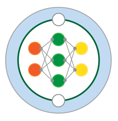
Dropout means randomly deactivating or temporarily removing some units from a layer of the network while training, along with all its incoming and outgoing connections. See more details here. It is usually the most useful regularization that we can do in fully connected layers.
In convolutional layers dropout makes less sense - see more discussion here
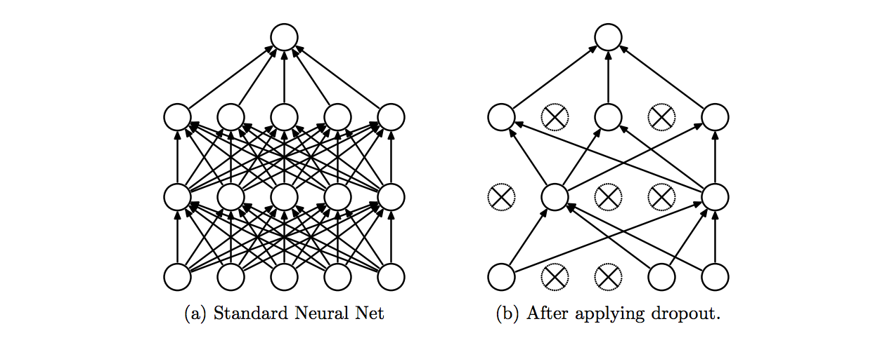
Fig. 4 Dropout Neural Net Model. Left: A standard neural net with 2 hidden layers. Right: An example of a thinned net produced by applying dropout to the network on the left. Crossed units have been dropped. Image taken from here.#
In the network defined below, we add dropout to with a probability of 20% to each layer. This means that during each training step, random 20% of the units within each layer will be deactivated.
class NetANNDropout(nn.Module):
    def __init__(self, dropout_rate=0.2):
        super().__init__()
        self.linear1 = nn.Linear(8, 16)
        self.linear2 = nn.Linear(16, 16)
        self.linear3 = nn.Linear(16, 8)

        self.dropout = nn.Dropout(dropout_rate)  # Dropout regularization
        self.relu = nn.ReLU()

    def forward(self, x):
        x = self.relu(self.linear1(x))
        x = self.dropout(x)
        x = self.relu(self.linear2(x))
        x = self.dropout(x)
        x = self.linear3(x)
        return x
# Network with very high dropout
nn_3l_drop = NetANNDropout(dropout_rate=0.5)

criterion = torch.nn.MSELoss()
optimizer_drop = optim.Adam(nn_3l_drop.parameters(), lr=0.003)
train_loss_drop, val_loss_drop = fit_model(
    nn_3l_drop, criterion, optimizer_drop, loader_train, loader_test, n_epochs
)
Training completed in 0 seconds.
Plotting the training and validation loss curves.
plt.figure(dpi=150)
plt.plot(train_loss_drop, "r", label="Training loss, with dropout")
plt.plot(val_loss_drop, "r--", label="Validation loss, with dropout")
plt.legend();
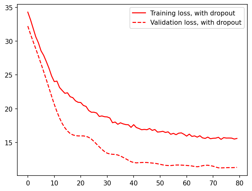
In this particular problem drop out does not seem to provide much advantage. While the model with drop out never seems to reach a state of overfitting (validation loss>training loss), it also does not perform as well as the model without any dropout.
Choosing the Learning Rate#
While training a neural network selecting a good learning rate (LR) is essential for both fast convergence and a lower error. A high learning rate can cause the training loss to never converge while a too small learning rate will cause the model to converge extremely slowly.
Finding the Optimal Learning Rate#
To choose the optimal learning rate for our network, we can use an LR finding algorithm. The objective of a LR Finder is to find the highest LR which still minimises the loss and does not make the loss diverge/explode. This is done by first starting with an extremely small LR and then increasing the LR after each batch until the corresponding loss starts to explode. To read more about learning rate finders, read this blog.
For our use case, we use the LR finder from the torch-lr-finder package to find the best learning rate for our neural network.
from torch_lr_finder import LRFinder
/usr/share/miniconda/envs/L96M2lines/lib/python3.9/site-packages/torch_lr_finder/lr_finder.py:5: TqdmExperimentalWarning: Using `tqdm.autonotebook.tqdm` in notebook mode. Use `tqdm.tqdm` instead to force console mode (e.g. in jupyter console)
  from tqdm.autonotebook import tqdm
Define the model and the optimizer. The optimizer is initialized with a very small learning rate.
nn_3l_lr = NetANN()
optimizer = optim.Adam(nn_3l_lr.parameters(), lr=1e-7)
Now we setup the LR finder and make it run for 200 iterations during which the learning rate varies from 1e-7 to 100.
lr_finder = LRFinder(nn_3l_lr, optimizer, criterion)
lr_finder.range_test(loader_train, end_lr=100, num_iter=200)
Stopping early, the loss has diverged
Learning rate search finished. See the graph with {finder_name}.plot()
Now we plot the LR vs the loss curve to find the best learning rate.
# Plot the lr vs the loss curve
lr_finder.plot()

# Reset the model and optimizer to their initial state
lr_finder.reset()
LR suggestion: steepest gradient
Suggested LR: 3.29E-02
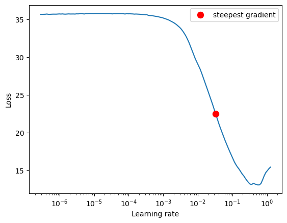
From the curve, we see that at the learning of approximately 0.01 we get the steepest gradient. So we choose 0.01 as the learning rate for our neural network.
n_epochs = 20
optimizer = optim.Adam(nn_3l_lr.parameters(), lr=0.01)

train_loss, val_loss = fit_model(
    nn_3l_lr, criterion, optimizer, loader_train, loader_test, n_epochs
)
Training completed in 0 seconds.
Plotting the training and validation loss curves.
plt.figure(dpi=150)
plt.plot(train_loss, "b", label="Training loss")
plt.plot(val_loss, "r", label="Validation loss")
plt.legend();
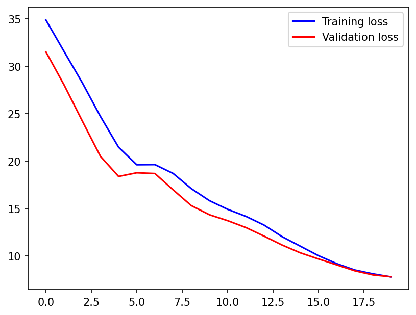
From the loss curves we can see that the loss has converged much faster than before.
Recommended Reading#
Batch Normalization#
Normalize the activation values such that the hidden representation don’t vary drastically and also helps to get improvement in the training speed.
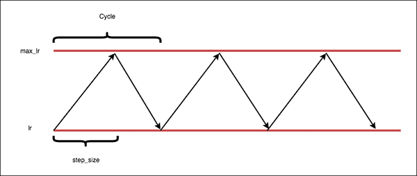
Cyclic learning rate#
The cyclic learning rate policy, introduced in Cyclical Learning Rates for Training Neural Networks, cycles the learning rate between two boundaries with a constant frequency in a triangular fashion. To read more about the cyclic learning rates and the one cycle policy, read here.
In PyTorch, cyclic learning rate can be used from optim.lr_scheduler.CyclicLR.