Using Neural Networks for L96 Parameterization: Online Testing#
Outline:#
In this notebook, we’ll extend upon the concepts learned in the previous notebook by implementing the neural networks as a parameterization in the single time scale Lorenz 96, and testing its impact in a simulation. Testing the impacts of parameterizations in a simulation is sometimes also referred to as online testing.
%matplotlib inline
import time

import matplotlib.pyplot as plt
import numpy as np
import torch
from torch import nn, optim
from torch.utils.data import TensorDataset, DataLoader

from L96_model import L96, RK4, L96_eq1_xdot
# Ensuring reproducibility
np.random.seed(14)
torch.manual_seed(14);
Load in the pre-trained parameterization networks#
We first load in the networks that were trained in the previous notebook.
linear_weights = torch.load("./networks/linear.pth")
local_FCNN_weights = torch.load("./networks/local_FCNN.pth")
nonlocal_FCNN_weights = torch.load("./networks/non_local_FCNN.pth")
We need to define the architecture that each model has before the weights can be assigned.
Show code cell content
# The model architectures
# ---------------------------


class LinearRegression(nn.Module):
    def __init__(self):
        super().__init__()
        self.linear1 = nn.Linear(1, 1)  # A single input and a single output

    def forward(self, x):
        # This method is automatically executed when
        # we call a object of this class
        x = self.linear1(x)
        return x


class FCNN(nn.Module):
    def __init__(self):
        super().__init__()
        self.linear1 = nn.Linear(1, 16)  # 8 inputs
        self.linear2 = nn.Linear(16, 16)
        self.linear3 = nn.Linear(16, 1)  # 8 outputs

        self.relu = nn.ReLU()

    def forward(self, x):
        x = self.relu(self.linear1(x))
        x = self.relu(self.linear2(x))
        x = self.linear3(x)
        return x


class NonLocal_FCNN(nn.Module):
    def __init__(self):
        super().__init__()
        self.linear1 = nn.Linear(8, 16)  # 8 inputs
        self.linear2 = nn.Linear(16, 16)
        self.linear3 = nn.Linear(16, 8)  # 8 outputs

        self.relu = nn.ReLU()

    def forward(self, x):
        x = self.relu(self.linear1(x))
        x = self.relu(self.linear2(x))
        x = self.linear3(x)
        return x
# Initialize network instances and assign pre-trained weights.
linear_network = LinearRegression()
linear_network.load_state_dict(linear_weights)

local_fcnn_network = FCNN()
local_fcnn_network.load_state_dict(local_FCNN_weights)

nonlocal_fcnn_network = NonLocal_FCNN()
nonlocal_fcnn_network.load_state_dict(nonlocal_FCNN_weights)
<All keys matched successfully>
Adding Parameterizations to GCM#
To recap, [Lorenz, 1995] describes a two-time scale dynamical system using two equations which are:
Note
All the GCM networks used in this notebook have been introduced earlier in notebooks Key aspects of GCMs parameterizations and Tuning GCM Parameterizations. To see the definition of those networks, expand the cells in the respective GCM sections below.
T_test = 10
forcing = 18
dt = 0.01

k = 8
j = 32

W = L96(k, j, F=forcing)

# Full L96 model (two time scale model)
X_full, _, _ = W.run(dt, T_test)
X_full = X_full.astype(np.float32)

init_conditions = X_full[0, :]
GCM Without Neural Network Parameterization#
Show code cell content
class GCM_without_parameterization:
    """GCM without parameterization

    Args:
        F: Forcing term
        time_stepping: Time stepping method
    """

    def __init__(self, F, time_stepping=RK4):
        self.F = F
        self.time_stepping = time_stepping

    def rhs(self, X, _):
        """Compute right hand side of the the GCM equations"""
        return L96_eq1_xdot(X, self.F)

    def __call__(self, X0, dt, nt, param=[0]):
        """Run GCM

        Args:
            X0: Initial conditions of X
            dt: Time increment
            nt: Number of forward steps to take
            param: Parameters of closure

        Returns:
            Model output for all variables of X at each timestep
            along with the corresponding time units
        """
        time, hist, X = (
            dt * np.arange(nt + 1),
            np.zeros((nt + 1, len(X0))) * np.nan,
            X0.copy(),
        )
        hist[0] = X

        for n in range(nt):
            X = self.time_stepping(self.rhs, dt, X, param)
            hist[n + 1], time[n + 1] = X, dt * (n + 1)
        return hist, time
gcm_no_param = GCM_without_parameterization(forcing)
X_no_param, t = gcm_no_param(init_conditions, dt, int(T_test / dt))
GCM With Neural Network Parameterization#
Show code cell content
class GCM_network:
    """GCM with neural network parameterization

    Args:
        F: Forcing term
        network: Neural network
        time_stepping: Time stepping method
    """

    def __init__(self, F, network, time_stepping=RK4):
        self.F = F
        self.network = network
        self.time_stepping = time_stepping

    def rhs(self, X, _):
        """Compute right hand side of the the GCM equations"""
        if self.network.linear1.in_features == 1:
            X_torch = torch.from_numpy(X)
            X_torch = torch.unsqueeze(X_torch, 1)
        else:
            X_torch = torch.from_numpy(np.expand_dims(X, 0))

        # Adding NN parameterization
        return L96_eq1_xdot(X, self.F) + np.squeeze(self.network(X_torch).data.numpy())

    def __call__(self, X0, dt, nt, param=[0]):
        """Run GCM

        Args:
            X0: Initial conditions of X
            dt: Time increment
            nt: Number of forward steps to take
            param: Parameters of closure

        Returns:
            Model output for all variables of X at each timestep
            along with the corresponding time units
        """
        time, hist, X = (
            dt * np.arange(nt + 1),
            np.zeros((nt + 1, len(X0))) * np.nan,
            X0.copy(),
        )
        hist[0] = X

        for n in range(nt):
            X = self.time_stepping(self.rhs, dt, X, param)
            hist[n + 1], time[n + 1] = X, dt * (n + 1)
        return hist, time
# Evaluate with linear network
gcm_linear_net = GCM_network(forcing, linear_network)
Xnn_linear, t = gcm_linear_net(init_conditions, dt, int(T_test / dt), linear_network)

# Evaluate with local FCNN
gcm_local_net = GCM_network(forcing, local_fcnn_network)
Xnn_local, t = gcm_local_net(init_conditions, dt, int(T_test / dt), local_fcnn_network)

# Evaluate with nonlocal FCNN
gcm_nonlocal_net = GCM_network(forcing, nonlocal_fcnn_network)
Xnn_nonlocal, t = gcm_nonlocal_net(
    init_conditions, dt, int(T_test / dt), nonlocal_fcnn_network
)
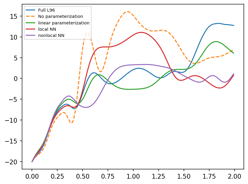
Comparing Results#
Comparing the predictions of GCM with different parameterizations.
time_i = 200
plt.figure(dpi=150)
plt.plot(t[:time_i], X_full[:time_i, 4], label="Full L96")
plt.plot(t[:time_i], X_no_param[:time_i, 4], "--", label="No parameterization")

plt.plot(t[:time_i], Xnn_linear[:time_i, 4], label="linear parameterization")

plt.plot(t[:time_i], Xnn_local[:time_i, 4], label="local NN")
plt.plot(t[:time_i], Xnn_nonlocal[:time_i, 4], label="nonlocal NN")
plt.legend(loc="upper left", fontsize=7);
Checking over many different initial conditions#
err_linear, err_local, err_nonlocal = [], [], []
T_test = 1

for i in range(90):
    init_conditions_i = X_full[i * 10, :]

    # Evaluate with linear network
    gcm_linear_net = GCM_network(forcing, linear_network)
    Xnn_linear, t = gcm_linear_net(
        init_conditions_i, dt, int(T_test / dt), linear_network
    )

    # Evaluate with local FCNN
    gcm_local_net = GCM_network(forcing, local_fcnn_network)
    Xnn_local, t = gcm_local_net(
        init_conditions_i, dt, int(T_test / dt), local_fcnn_network
    )

    # Evaluate with nonlocal FCNN
    gcm_nonlocal_net = GCM_network(forcing, nonlocal_fcnn_network)
    Xnn_nonlocal, t = gcm_nonlocal_net(
        init_conditions_i, dt, int(T_test / dt), nonlocal_fcnn_network
    )

    # GCM parameterized by the global 3-layer network
    # gcm_net_3layers = GCM_network(forcing, nn_3l)
    # Xnn_3layer_i, t = gcm_net_3layers(init_conditions_i, dt, int(T_test / dt), nn_3l)

    # GCM parameterized by the linear network
    # gcm_net_1layers = GCM_network(forcing, linear_network)
    # Xnn_1layer_i, t = gcm_net_1layers(init_conditions_i, dt, int(T_test / dt), linear_network)

    err_linear.append(
        np.sum(np.abs(X_full[i * 10 : i * 10 + T_test * 100 + 1] - Xnn_linear))
    )

    err_local.append(
        np.sum(np.abs(X_full[i * 10 : i * 10 + T_test * 100 + 1] - Xnn_local))
    )

    err_nonlocal.append(
        np.sum(np.abs(X_full[i * 10 : i * 10 + T_test * 100 + 1] - Xnn_nonlocal))
    )


print(f"Sum of errors for linear: {sum(err_linear):.2f}")
print(f"Sum of errors for local neural network: {sum(err_local):.2f}")
print(f"Sum of errors for non-local neural network: {sum(err_nonlocal):.2f}")
Sum of errors for linear: 53703.23
Sum of errors for local neural network: 31679.62
Sum of errors for non-local neural network: 40778.95
In this evaluation we see that the neural networks perform much better than the linear model. However, incorporating non-locality did not improve model performance over the local model. It may be possible to have improved this by building a better non-local model by a larger parameter sweep.
Summary#
In this notebook we showed how neural networks can be added as a parameterization to the single timescale L96 model (the gcm analogue of the two timescale L96 model). The neural network parameterizations performed better than the linear parameterization, as shown by evaluating the model performance over many initial conditions.
In these notebook we have followed the strategy of :
running a realistic (more time scales resolved) simulation.
evaluating the impact of the fast scales (which could not be resolved if the simulation resolved fewer time scales) on the slow scales in the realistic simulation.
learning a functional relationship between the impact of the fast scales on the slow scale and the slow scales.
incoporating this relationship (ML based parameterization) in the model of the slow time scales, and evaluating the success (if any).
This is a strategy of offline training and online testing.
A different strategy to have would have been to not necessarily learn the impact of or the patterns in the sub-grid scales. But rather optimize a model such that when it is added to the slow time scale model, it leads to the time evolution of the slow time scale model being closer to the two time scale model (which is our ultimate goal). This strategy is sometimes called online training, and discussed in the next notebook. A short primer to this was presented in the notebook on gcm tuning, where we tuned parameters to match the time evolution of the more realistic model.