Gaussian Processes#
import numpy as np
import matplotlib.pyplot as plt
import tensorflow as tf
import gpflow
from L96_model import L96, L96_eq1_xdot, integrate_L96_2t
from L96_model import EulerFwd, RK2, RK4
import os

os.environ["TF_USE_LEGACY_KERAS"] = "True"

time_method = RK4
2024-10-12 17:40:58.043939: I external/local_xla/xla/tsl/cuda/cudart_stub.cc:32] Could not find cuda drivers on your machine, GPU will not be used.
2024-10-12 17:40:58.047042: I external/local_xla/xla/tsl/cuda/cudart_stub.cc:32] Could not find cuda drivers on your machine, GPU will not be used.
2024-10-12 17:40:58.055942: E external/local_xla/xla/stream_executor/cuda/cuda_fft.cc:485] Unable to register cuFFT factory: Attempting to register factory for plugin cuFFT when one has already been registered
2024-10-12 17:40:58.070076: E external/local_xla/xla/stream_executor/cuda/cuda_dnn.cc:8454] Unable to register cuDNN factory: Attempting to register factory for plugin cuDNN when one has already been registered
2024-10-12 17:40:58.074200: E external/local_xla/xla/stream_executor/cuda/cuda_blas.cc:1452] Unable to register cuBLAS factory: Attempting to register factory for plugin cuBLAS when one has already been registered
2024-10-12 17:40:58.085434: I tensorflow/core/platform/cpu_feature_guard.cc:210] This TensorFlow binary is optimized to use available CPU instructions in performance-critical operations.
To enable the following instructions: AVX2 FMA, in other operations, rebuild TensorFlow with the appropriate compiler flags.
2024-10-12 17:40:58.838296: W tensorflow/compiler/tf2tensorrt/utils/py_utils.cc:38] TF-TRT Warning: Could not find TensorRT
Recap: Lorenz 96#

Fig. 9 Visualisation of a two-scale Lorenz ‘96 system with J = 8 and K = 6. Global-scale variables (\(X_k\)) are updated based on neighbouring variables and on the local-scale variables (\(Y_{j,k}\)) associated with the corresponding global-scale variable. Local-scale variabless are updated based on neighbouring variables and the associated global-scale variable. The neighbourhood topology of both local and global-scale variables is circular. Image from Exploiting the chaotic behaviour of atmospheric models with reconfigurable architectures - Scientific Figure on ResearchGate..#
[Lorenz, 1995] describes a “two time-scale” model in two equations (2 and 3) which are:
Recap: Gaussian Processes (GPs)#
Exact inference#
Consider the following case where we have a dataset \(\mathcal{D}\) comprising \(n\) pairs of observations \(\mathcal{D} = \{(x_1,y_1),(x_2,y_2),...,(x_n,y_n)\}\), where \(x_i\) could e.g., be the coarse-grid term at time \(i\) and \(y_i\) the corresponding sub-grid term. In the standard supervised learning problem, we wish to recover the function \(f\) which maps a given input \(x_i\) to a given output \(y_i\), where we assume that the outputs have been corrupted by some random noise \(\varepsilon_i\):
or in vector format:
Then after learning the function \(f\), we wish to make reliable predictions at un-observed test input locations \(\textbf{x}_* \in \mathbb{R}^{n_*}\), such that:
In the GP framework, we assume that the noise term \(\pmb{\varepsilon}\) represents independent and identically distributed zero-mean Gaussian noise, with variance \(\sigma^2\), such that \(\varepsilon_i \sim \mathcal{N}(0,\sigma^2)\), and that the function \(f\) itself is a GP:
where \(m(\pmb{\phi})\) and \(k(\pmb{\phi},\pmb{\phi})\) are the mean and covariance (or kernel) of the GP respectively, and \(\pmb{\phi}\) represents arbitrary function inputs - either \(\textbf{x}\) or \(\textbf{x}_*\). Through the assumption that \(f\) is a GP, we effectively place prior probabilities over all conceviable functions \(f_i\), where \(i = \{1,2,...,\infty\}\), but assign higher probabilities to specific types of functions (e.g., linear, periodic, anisotropic, non-stationary etc) through our choice of \(m(\pmb{\phi})\) and \(k(\pmb{\phi},\pmb{\phi})\). After which, we use the observations \(\textbf{y}\) to update these prior probabilities in the form of a posterior distribution over functions. Let’s see how we do this in practice:
Continuing with the notation that \(\textbf{x} = \{x_1,x_2,...,x_n\}\) represents the set of training inputs, and \(\textbf{x}_* = \{x_{*_1},x_{*_2},...,x_{*_{n_*}}\}\) the set of test inputs, we wish to train a model which is able to make accurate predictions at the test locations: \(\textbf{f}_* = \{f(x_{*_1}),f(x_{*_2}),...,f(x_{*_{n_*}})\}\). We start by defining a series of covariance functions associated with the training and test inputs:
The covariance function of the GP prior is a particularly important concept, as this is what allows us to model the different kinds of functions described above, so consideration should go into choosing the most appropriate function (there are data driven ways to make this choice. We could e.g., use cross-validation, or more commonly in Bayesian statistics; compare models via the log marginal likelihood - GPflow is setup to do the latter). Now, because a GP can ultimately be described as a collection of random Gaussian variables, under our GP prior (defined by \(m(\pmb{\phi})\) and \(k(\pmb{\phi},\pmb{\phi})\)), the function values \(\textbf{f}_*\) and the training observations \(\textbf{y}\) are considered to form a joint Gaussian distribution:
where we see that the marginal distributions (under the prior) of both \(\textbf{f}_*\) and \(\textbf{y}\) are given by:
In reality however, we are interested in the conditional distribution of the function values, given the training data - \(p(\textbf{f}_* | \textbf{y},\textbf{x},\textbf{x}_*)\), which is also Gaussian such that \(\textbf{f}_* | \textbf{y},\textbf{x},\textbf{x}_* \sim \mathcal{N}(\bar{\textbf{f}}_*,\sigma^2_{\textbf{f}_*})\). The mean and covariance of this distribution then tells us everything we need about the posterior distribution of the function values, and can be derived analytically through a bit of linear algebra (see [Rasmussen and Williams, 2005] or [Bishop, 2006] for details). Here is the final solution:
Variational inference#
The analytical solution in the above description relies on the assumption that the data are Gaussian distributed, which makes the maths straightfoward because the product of 2 Gaussians (the prior and likelihood) results in another Gaussian (the posterior). In the case where the data are not Gaussian distributed, the resultant posterior will no longer have a closed-form solution, so instead we need to approximate the posterior as a multivarite Gaussian (or other) using variational techniques. To do this, GPflow implements the approach outlined in Opper and Archambeau, (2009), and we give a brief summary here to follow on from the section above.
Recall the posterior predictive distribution from before: \(p(\textbf{f}_* | \textbf{y})\), where we have removed the dependence on the inputs \(\textbf{x}\) and \(\textbf{x}_*\) to keep the notation uncluttered. In the following discussion we assume that this distribution is no longer Gaussian, because e.g., the observations \(\textbf{y}\) are no longer Gaussian, and hence we no longer have a Gaussian likelihood. Therefore instead, we wish to approximate \(p(\textbf{f}_* | \textbf{y})\) by a multivariate Gaussian \(q(\textbf{f}_*) \sim \mathcal{N}(\textbf{m},\textbf{S})\). This is achieved by choosing the values of \(\textbf{m}\) and \(\textbf{S}\) which minimise the variational free energy cost function:
where
is the marginal likelihood (the probability of the observations under the model prior; commonly referred to as the evidence), and
is the Kullback-Leibler divergence which compares the similarity of two probability distributions (in this case, \(q(\textbf{f}_*)\) and \(p(\textbf{f}_* | \textbf{y}\))).
The variational free energy \(\mathcal{J}\big(q(\textbf{f}_*)\big)\) represents an upper bound on the negative (log) evidence \(-\ln p(\textbf{y})\), and is the quantity that GPflow minimises in the variational setting. It is however common practice to track the maximisation of the negative variational free energy, which then represents a lower bound on the (log) evidence, known as the Evidence Lower BOund (ELBO):
Once the values of \(\textbf{m}\) and \(\textbf{S}\) have been optimised, the Gaussian approximation for the mean and covariance of the posterior can be computed as:
Note that in practice there is a fair bit of maths involved in computing \(\mathcal{J}\big(q(\textbf{f}_*)\big)\) which we do not show here, however the reader is referred to the GPflow docs and the Opper and Archambeau, (2009) paper for more information. See also this nice Jupyter notebook workthrough by So Takao from the University College London Centre for AI, which includes the derivations of the KL divergence term in the Appendix.
Sparse GPs#
Due to the need to invert the kernel matrix \(\textbf{K}\) (which has size \(n \times n\)) in both the exact and variational settings, GP problems scale with complexity \(\mathcal{O}(n^3)\). Therefore for data sets with more than a few thousand training points, the standard GP implementations above become problematic. A solution to this is to consider sparse GPs which rely on a set of inducing variables to learn the function \(f\), as outlined in Titsias, (2009). Note that GPflow has 2 commonly used classes for implementation of the inducing points method, namely ‘SGPR’ and ‘SVGP’. Although at first it perhaps may seem that ‘SVGP’ is for variational inference and ‘SGPR’ is for exact inference, this is not actually the case. Sparse learning requires variational inference in either case, it is just that ‘SVGP’ is used for non-Gaussian data (as described above), while ‘SGPR’ is used for Gaussian data. Let’s introduce the inducing points method now:
Consider the set of points \(\textbf{z} = \{z_1,z_2,...,z_m\}\) where \(m << n\), which could perhaps correspond to a subset of the training inputs, or a hold-out set etc, however the important point is that they exist in the same space as the inputs. These points are known as the inducing points, and subsequently their corresponding latent function values \(\textbf{u} = \{f(z_1),f(z_2),...,f(z_m)\}\) are known as the inducing variables. If we then assume that the posterior predictive function values at the input locations \(\textbf{x}\) and \(\textbf{x}_*\) (given by \(\textbf{f}\) and \(\textbf{f}_*\) respectively) are conditionally independent given \(\textbf{u}\), we can describe the posterior \(p(\textbf{f}_* | \textbf{y})\) as a function of \(\textbf{u}\) as follows:
We can subsequently derive an analytical solution for \(p(\textbf{f}_* | \textbf{u})\) above by recalling in the first section on exact inference how \(\textbf{y}\) and \(\textbf{f}_*\) formed a joint Gaussian under the GP prior. The same principles apply here to \(\textbf{u}\) and \(\textbf{f}_*\), hence the mean and covariance of \(p(\textbf{f}_* | \textbf{u})\) follows the same form as those defined by \(\bar{\textbf{f}}_*\) and \(\sigma_{\textbf{f}_*}\) previously, except this time we replace all occurrences of \(\textbf{x}\) with \(\textbf{z}\), as well as re-defining the covariance matrices:
The second distribution above, \(p(\textbf{u} | \textbf{y})\), does not have a closed-form solution however, so we need to rely on variational inference to approximate it as a multivariate Gaussian \(q(\textbf{u}) \sim \mathcal{N}(\textbf{m},\textbf{S})\). Similar to what we saw in the variational inference discussion above, both \(\textbf{m}\) and \(\textbf{S}\) (as well as \(\textbf{z}\)) can be optimised by minimising the variational free energy cost function \(\mathcal{J}\big(q(\textbf{f}_*)\big)\). After which, we can produce an analytical solution for the approximate posterior mean and covariance as we have already seen, by once again replacing all occurrences of \(\textbf{x}\) with \(\textbf{z}\), as well as re-defining the covariance matrices. This results in much cheaper inference than before as the covariance matrix \(\textbf{K}\) is now of size \(m \times m\), hence the computational cost of the matrix inverse is now \(\mathcal{O}(m^3)\) as opposed to \(\mathcal{O}(n^3)\).
# - a GCM class without any parameterization
class GCM_no_param:
def __init__(self, F, time_stepping=time_method):
self.F = F
self.time_stepping = time_stepping
def rhs(self, X, param):
return L96_eq1_xdot(X, self.F)
def __call__(self, X0, dt, nt, param=[0]):
# X0 - initial conditions, dt - time increment, nt - number of forward steps to take
# param - parameters of our closure
time, hist, X = (
dt * np.arange(nt + 1),
np.zeros((nt + 1, len(X0))) * np.nan,
X0.copy(),
)
hist[0] = X
for n in range(nt):
X = self.time_stepping(self.rhs, dt, X, param)
hist[n + 1], time[n + 1] = X, dt * (n + 1)
return hist, time
# - a GCM class including a linear parameterization in rhs of equation for tendency
class GCM:
def __init__(self, F, parameterization, time_stepping=time_method):
self.F = F
self.parameterization = parameterization
self.time_stepping = time_stepping
def rhs(self, X, param):
return L96_eq1_xdot(X, self.F) - self.parameterization(param, X)
def __call__(self, X0, dt, nt, param=[0]):
# X0 - initial conditions, dt - time increment, nt - number of forward steps to take
# param - parameters of our closure
time, hist, X = (
dt * np.arange(nt + 1),
np.zeros((nt + 1, len(X0))) * np.nan,
X0.copy(),
)
hist[0] = X
for n in range(nt):
X = self.time_stepping(self.rhs, dt, X, param)
hist[n + 1], time[n + 1] = X, dt * (n + 1)
return hist, time
# - a GCM class including a GP parameterization in rhs of equation for tendency
class GCM_GP:
def __init__(self, F, GP, time_stepping=time_method, stochastic=True, local=True):
self.F = F
self.GP = GP
self.time_stepping = time_stepping
self.stochastic = stochastic
self.local = local
def rhs(self, X, param):
if self.local: # i.e. outputs are shape n*K
X_ten = tf.convert_to_tensor(np.atleast_2d(X).T, dtype=tf.float64)
else: # i.e. outputs are shape n x K
X_augment = np.hstack((np.atleast_2d(X).T, np.atleast_2d(np.arange(K)).T))
X_ten = tf.convert_to_tensor(X_augment, dtype=tf.float64)
if self.stochastic:
f_mean = self.GP.predict_f_samples(
X_ten, 1
) # produce 1 random sample from the posterior over functions
else:
f_mean, f_variance = self.GP.predict_f(X_ten)
return L96_eq1_xdot(X, self.F) + np.squeeze(f_mean)
def __call__(self, X0, dt, nt, param=[0]):
# X0 - initial conditions, dt - time increment, nt - number of forward steps to take
# param - parameters of our closure
time, hist, X = (
dt * np.arange(nt + 1),
np.zeros((nt + 1, len(X0))) * np.nan,
X0.copy(),
)
hist[0] = X
for n in range(nt):
X = self.time_stepping(self.rhs, dt, X, param)
hist[n + 1], time[n + 1] = X, dt * (n + 1)
return hist, time
# Define the function which will be used to track the optimisation of the models. Much of the code in the 'GP'
# function is borrowed from the example on the GPflow website:
# https://gpflow.github.io/GPflow/2.4.0/notebooks/advanced/gps_for_big_data.html
def trainGP(
model,
training_data=None,
validation_data=None,
batch_size=None,
iterations=1000,
verbose=0,
):
tf.random.set_seed(766)
n = len(training_data[0])
if batch_size is None:
batch_size = n
train_dataset = (
tf.data.Dataset.from_tensor_slices(training_data).repeat().shuffle(1000)
)
train_iter = iter(train_dataset.batch(batch_size))
training_loss = model.training_loss_closure(train_iter, compile=True)
optimizer = tf.keras.optimizers.legacy.Adam()
@tf.function
def optimization_step(trainable_variables):
optimizer.minimize(training_loss, trainable_variables)
elbo_log = []
iters = []
pred_error = []
for step in range(iterations):
optimization_step(model.trainable_variables)
if step % 10 == 0:
loss = -training_loss().numpy()
prediction, uncertainty = model.predict_f(validation_data[0])
pred_error.append(np.mean((prediction - validation_data[1]) ** 2))
elbo_log.append(loss)
iters.append(step)
if verbose > 0:
if step < 1000:
if step % 100 == 0:
print(f"ELBO at step {step}: {loss:.2f}")
else:
if step % 1000 == 0:
print(f"ELBO at step {step}: {loss:.2f}")
return model, iters, elbo_log, pred_error
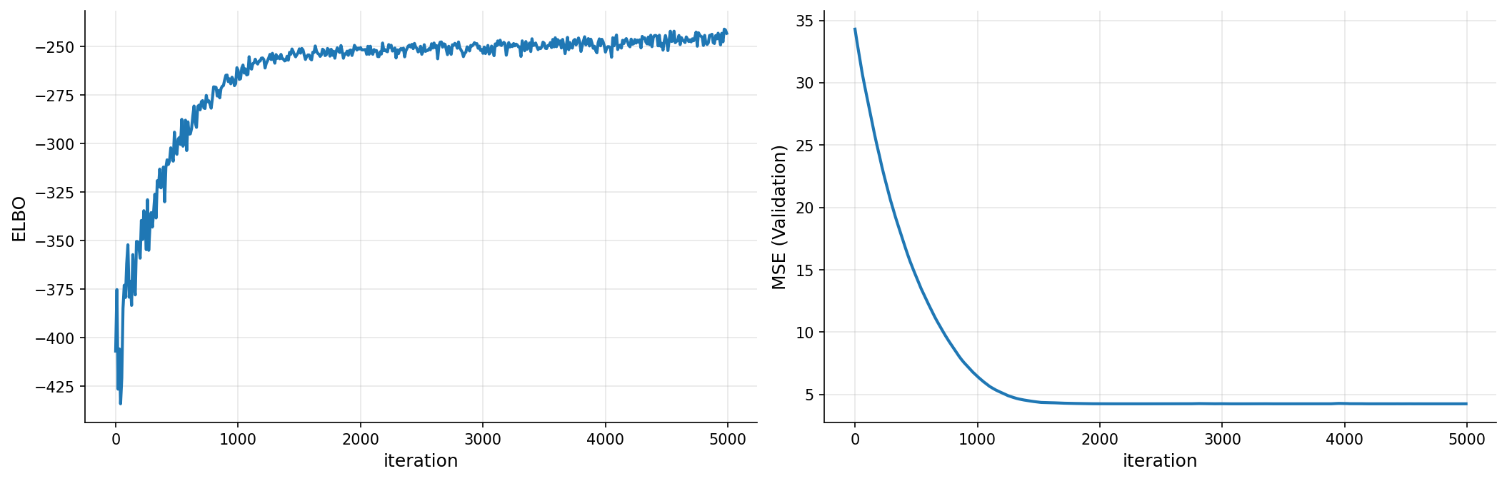
def plot_loss(x, train, valid, labels=["ELBO", "MSE (Validation)"]):
fig, ax = plt.subplots(1, 2, figsize=(17, 5), dpi=150)
plots = [train, valid]
for c in range(2):
ax[c].spines["top"].set_color(None)
ax[c].spines["right"].set_color(None)
ax[c].plot(x, plots[c], lw=2)
ax[c].set_xlabel("iteration", fontsize=12)
ax[c].set_ylabel(labels[c], fontsize=12)
ax[c].grid(True, alpha=0.3)
plt.subplots_adjust(wspace=0.1)
plt.show()
Learn the sub-grid tendencies offline#
time_steps = 20000
Forcing, dt, T = 18, 0.01, 0.01 * time_steps

# Create a "real world" with K=8 and J=32
W = L96(8, 32, F=Forcing)
# Get training and validation data for the GP model
val_size = 4000

# - Run the true state and output subgrid tendencies (the effect of Y on X is xytrue):
Xtrue, _, _, xytrue = W.run(dt, T, store=True, return_coupling=True)
gcm_no_param = GCM_no_param(Forcing)

# train:
X_train = Xtrue[:-val_size, :]
Y_train = xytrue[:-val_size, :]

# test:
X_valid = Xtrue[-val_size:, :]
Y_valid = xytrue[-val_size:, :]

n, K = Y_train.shape
ns = len(X_valid)
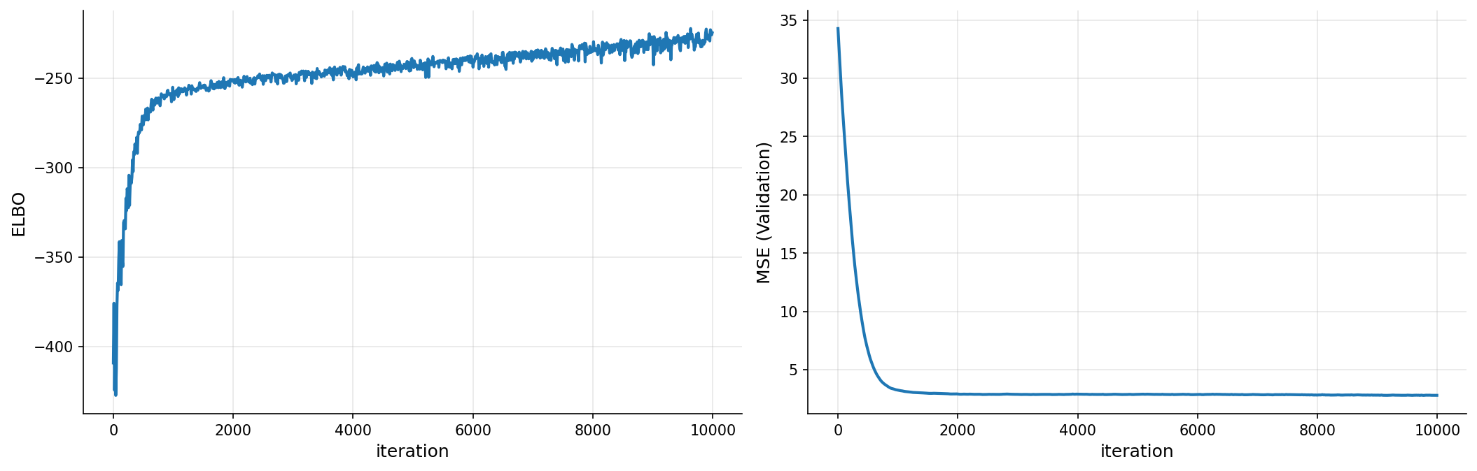
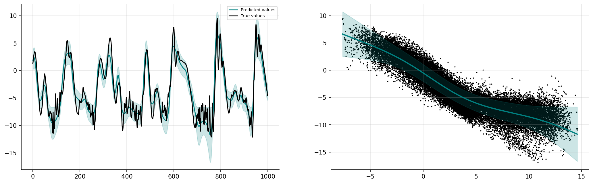
Local mappings with a linear kernel#
The linear GP kernel is equivalent to:
\(k(\textbf{x},\textbf{x}') = \theta^2 \big(\textbf{x}\textbf{x}'^\text{T}\big)\), where \(\theta\) is a tunable hyperparameter.
First we will build a GP with a linear kernel while assuming the outputs (i.e., each of the Ks) are independent. The extension to learning non-linear functions is trivial. We simply define a new kernel, e.g., gpflow.kernels.Matern32(). Incorporating non-local information (i.e., from other ks (we have 8 ks in total)) is a little more tricky, but we will tackle this later.
np.random.seed(2)

x_train = tf.convert_to_tensor(X_train.reshape(n * K, 1, order="F"), dtype=tf.float64)
y_train = tf.convert_to_tensor(Y_train.reshape(n * K, 1, order="F"), dtype=tf.float64)
x_valid = tf.convert_to_tensor(X_valid.reshape(ns * K, 1, order="F"), dtype=tf.float64)
y_valid = Y_valid.reshape(ns * K, 1, order="F")

M = 50  # number of inducing variables
Z = tf.convert_to_tensor(
    np.atleast_2d(np.linspace(np.min(x_train), np.max(x_train), M)).T, dtype=tf.float64
)

kernel = gpflow.kernels.Linear()
lik = gpflow.likelihoods.Gaussian()
gp_linear = gpflow.models.SVGP(kernel=kernel, likelihood=lik, inducing_variable=Z)
gp_linear.likelihood.variance.assign(np.var(y_train))
gp_linear, iters, elbo, pred_error = trainGP(
    gp_linear,
    training_data=(x_train, y_train),
    validation_data=(x_valid, y_valid),
    iterations=5000,
    batch_size=100,
    verbose=0,
)
plot_loss(iters, elbo, pred_error)
gp_linear
| name | class | transform | prior | trainable | shape | dtype | value |
|---|---|---|---|---|---|---|---|
| SVGP.kernel.variance | Parameter | Softplus | True | () | float64 | 0.9922619440901339 | |
| SVGP.likelihood.variance | Parameter | Softplus + Shift | True | () | float64 | 15.46902 | |
| SVGP.inducing_variable.Z | Parameter | Identity | True | (50, 1) | float64 | [[-14.51073... | |
| SVGP.q_mu | Parameter | Identity | True | (50, 1) | float64 | [[9.50147776e-01... | |
| SVGP.q_sqrt | Parameter | FillTriangular | True | (1, 50, 50) | float64 | [[[6.80571681e-02, 0.00000000e+00, 0.00000000e+00... |
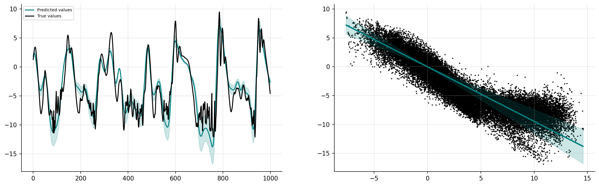
prediction_linGP, uncertainty_linGP = gp_linear.predict_f(x_valid)
prediction_linGP = np.squeeze(prediction_linGP.numpy())
uncertainty_linGP = np.squeeze(uncertainty_linGP.numpy())

n_std = 3
start = 31000
end = start + 1000
prediction_linGPplot = prediction_linGP[start:end]
uncertainty_linGPplot = n_std * np.sqrt(uncertainty_linGP[start:end])

fig, ax = plt.subplots(1, 2, figsize=(17, 5), dpi=150)
ax[0].spines["top"].set_color(None)
ax[0].spines["right"].set_color(None)
ax[0].plot(prediction_linGPplot, label="Predicted values", color="teal")
ax[0].fill_between(
    np.arange(1000),
    prediction_linGPplot + uncertainty_linGPplot,
    prediction_linGPplot - uncertainty_linGPplot,
    alpha=0.2,
    color="teal",
)
ax[0].plot(y_valid[start:end], label="True values", color="k")
ax[0].grid(True, alpha=0.3)
ax[0].legend(fontsize=7)

a, b = zip(*sorted(zip(X_valid.reshape(ns * K, order="F"), prediction_linGP)))
a, c = zip(
    *sorted(zip(X_valid.reshape(ns * K, order="F"), n_std * np.sqrt(uncertainty_linGP)))
)
a = np.array(a)
b = np.array(b)
c = np.array(c)

ax[1].spines["top"].set_color(None)
ax[1].spines["right"].set_color(None)
ax[1].scatter(
    X_valid.reshape(ns * K, order="F"),
    Y_valid.reshape(ns * K, order="F"),
    s=1,
    color="k",
)
ax[1].plot(X_valid.reshape(ns * K, order="F"), prediction_linGP, color="teal", lw=2)
ax[1].fill_between(a, b - c, b + c, color="teal", alpha=0.2)
ax[1].grid(True, alpha=0.3)
plt.show()
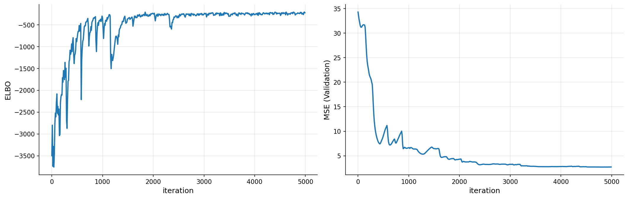
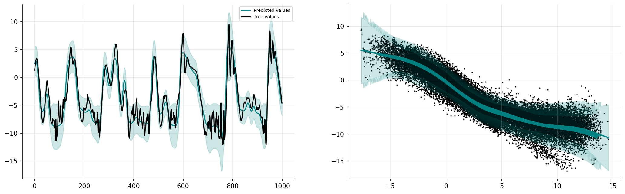
Local mappings with a non-linear kernel#
Here we are going to opt for a combination of 2 kernels: The Rational Quadratic kernel:
\(k_1(\textbf{x},\textbf{x}') = \theta_1^2 \bigg(1 + \dfrac{\Vert \textbf{x} - \textbf{x}' \Vert^2}{2\theta_2^2\theta_3}\bigg)^{-\theta_3}\)
and the linear kernel:
\(k_2(\textbf{x},\textbf{x}') = \theta_4^2 \big(\textbf{x}\textbf{x}^\text{T}\big)\)
such that our kernel becomes \(k(\textbf{x},\textbf{x}') = k_1(\textbf{x},\textbf{x}') + k_2(\textbf{x},\textbf{x}')\)
np.random.seed(2)

x_train = tf.convert_to_tensor(X_train.reshape(n * K, 1, order="F"), dtype=tf.float64)
y_train = tf.convert_to_tensor(Y_train.reshape(n * K, 1, order="F"), dtype=tf.float64)
x_valid = tf.convert_to_tensor(X_valid.reshape(ns * K, 1, order="F"), dtype=tf.float64)
y_valid = Y_valid.reshape(ns * K, 1, order="F")

M = 50  # number of inducing variables
Z = tf.convert_to_tensor(
    np.atleast_2d(np.linspace(np.min(x_train), np.max(x_train), M)).T, dtype=tf.float64
)

kernel = gpflow.kernels.RationalQuadratic() + gpflow.kernels.Linear()
lik = gpflow.likelihoods.Gaussian()
gp_nonlinear = gpflow.models.SVGP(kernel=kernel, likelihood=lik, inducing_variable=Z)
gp_nonlinear.likelihood.variance.assign(np.var(y_train))
gp_nonlinear, iters, elbo, pred_error = trainGP(
    gp_nonlinear,
    training_data=(x_train, y_train),
    validation_data=(x_valid, y_valid),
    iterations=10000,
    batch_size=100,
    verbose=0,
)
plot_loss(iters, elbo, pred_error)
gp_nonlinear
| name | class | transform | prior | trainable | shape | dtype | value |
|---|---|---|---|---|---|---|---|
| SVGP.kernel.kernels[0].variance | Parameter | Softplus | True | () | float64 | 1.74892 | |
| SVGP.kernel.kernels[0].lengthscales | Parameter | Softplus | True | () | float64 | 3.69422 | |
| SVGP.kernel.kernels[0].alpha | Parameter | Softplus | True | () | float64 | 3.13103 | |
| SVGP.kernel.kernels[1].variance | Parameter | Softplus | True | () | float64 | 0.8428626627224527 | |
| SVGP.likelihood.variance | Parameter | Softplus + Shift | True | () | float64 | 9.71508 | |
| SVGP.inducing_variable.Z | Parameter | Identity | True | (50, 1) | float64 | [[-14.40122... | |
| SVGP.q_mu | Parameter | Identity | True | (50, 1) | float64 | [[9.04107705e-01... | |
| SVGP.q_sqrt | Parameter | FillTriangular | True | (1, 50, 50) | float64 | [[[1.69896241e-01, 0.00000000e+00, 0.00000000e+00... |
prediction_nonlinGP, uncertainty_nonlinGP = gp_nonlinear.predict_f(x_valid)
prediction_nonlinGP = np.squeeze(prediction_nonlinGP.numpy())
uncertainty_nonlinGP = np.squeeze(uncertainty_nonlinGP.numpy())

n_std = 3
start = 31000
end = start + 1000
prediction_nonlinGPplot = prediction_nonlinGP[start:end]
uncertainty_nonlinGPplot = n_std * np.sqrt(uncertainty_nonlinGP[start:end])

fig, ax = plt.subplots(1, 2, figsize=(17, 5), dpi=150)
ax[0].spines["top"].set_color(None)
ax[0].spines["right"].set_color(None)
ax[0].plot(prediction_nonlinGPplot, label="Predicted values", color="teal")
ax[0].fill_between(
    np.arange(1000),
    prediction_nonlinGPplot + uncertainty_nonlinGPplot,
    prediction_nonlinGPplot - uncertainty_nonlinGPplot,
    alpha=0.2,
    color="teal",
)
ax[0].plot(y_valid[start:end], label="True values", color="k")
ax[0].grid(True, alpha=0.3)
ax[0].legend(fontsize=7)

a, b = zip(*sorted(zip(X_valid.reshape(ns * K, order="F"), prediction_nonlinGP)))
a, c = zip(
    *sorted(
        zip(X_valid.reshape(ns * K, order="F"), n_std * np.sqrt(uncertainty_nonlinGP))
    )
)
a = np.array(a)
b = np.array(b)
c = np.array(c)

ax[1].spines["top"].set_color(None)
ax[1].spines["right"].set_color(None)
ax[1].scatter(
    X_valid.reshape(ns * K, order="F"),
    Y_valid.reshape(ns * K, order="F"),
    s=1,
    color="k",
)
ax[1].plot(a, b, color="teal", lw=2)
ax[1].fill_between(a, b - c, b + c, color="teal", alpha=0.2)
ax[1].grid(True, alpha=0.3)
plt.show()
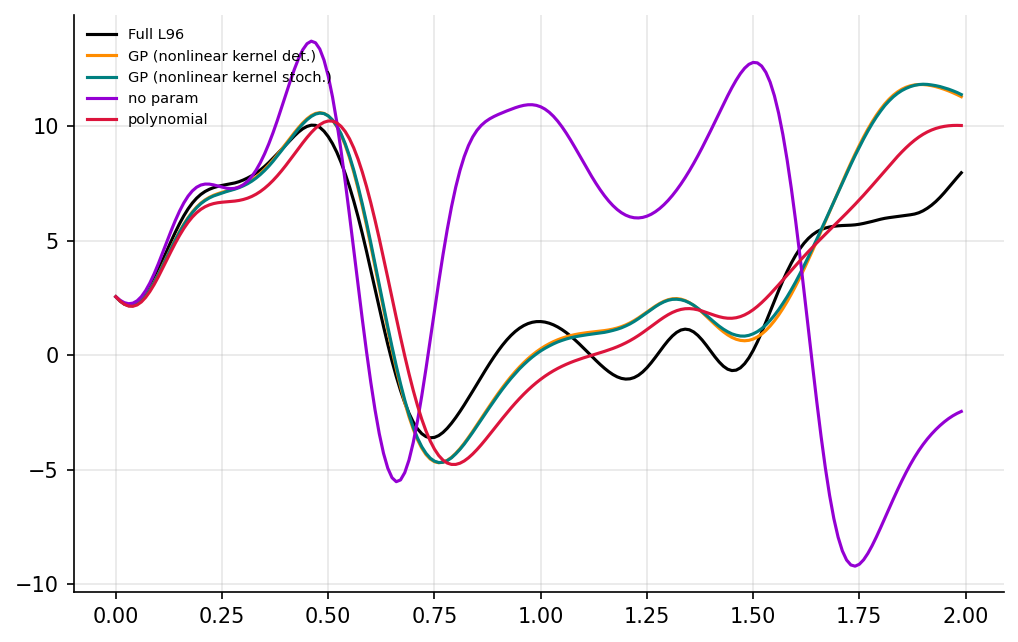
Implement the linear GP parameterisation in an online setting#
T_test = 10

X_full, _, _, _ = W.run(dt, T_test, return_coupling=True)  # Full model

init_cond = Xtrue[-1, :]

gcm_gp_det = GCM_GP(Forcing, gp_nonlinear, stochastic=False)
Xgp_det, t = gcm_gp_det(init_cond, dt, int(T_test / dt), gp_nonlinear)

gcm_gp_sto = GCM_GP(Forcing, gp_nonlinear, stochastic=True)
Xgp_sto, t = gcm_gp_sto(init_cond, dt, int(T_test / dt), gp_nonlinear)

gcm_no_param = GCM_no_param(Forcing)
X_no_param, t = gcm_no_param(init_cond, dt, int(T_test / dt))

naive_parameterization = lambda param, X: np.polyval(param, X)
gcm = GCM(Forcing, naive_parameterization)
X_param, t = gcm(init_cond, dt, int(T / dt), param=[0.85439536, 1.75218026])

time_i = 200
fig, ax = plt.subplots(1, figsize=(8, 5), dpi=150)
ax.spines["top"].set_color(None)
ax.spines["right"].set_color(None)
ax.plot(t[:time_i], X_full[:time_i, 4], label="Full L96", color="k")
ax.plot(
    t[:time_i],
    Xgp_det[:time_i, 4],
    label="GP (nonlinear kernel det.)",
    color="darkorange",
)
ax.plot(
    t[:time_i], Xgp_sto[:time_i, 4], label="GP (nonlinear kernel stoch.)", color="teal"
)
ax.plot(t[:time_i], X_no_param[:time_i, 4], label="no param", color="darkviolet")
ax.plot(t[:time_i], X_param[:time_i, 4], label="polynomial", color="crimson")
ax.grid(True, alpha=0.3)
plt.legend(frameon=False, loc="upper left", fontsize=7)
plt.show()
Use multi-task GPs to exploit non-local features#
In the GP literature, it is common to see the multi-task learning problem framed the same set of inputs are used to learn each of the functional mappings to the various outputs:
however it is also possible to define a unique set of inputs which map to the corresponding \(k\), i.e:
This is more applicable to our case as we have 8 coarse grid terms, each of which map to their own respective sub-grid terms. We then want to model for any potential correlation between the outputs \(\textbf{y}_k\), and hence the various functions \(f_k(\textbf{x}_k)\). One way to achieve this is through a concept known as Linear models for coregionalisation (see e.g., Álvarez et al, 2012), where we assume that the function \(f(\textbf{x})\) is drawn from the linear combination of some latent function \(g(\textbf{x})\), such that:
where \(f(\textbf{x}) \in \mathbb{R}^K\), \(g(\textbf{x}) \in \mathbb{R}^L\), and \(\textbf{W} \in \mathbb{R}^{K \times L}\), where \(L \leq K\). The principle is that the outputs of \(g(\textbf{x})\) are uncorrelated, but through combining them with \(\textbf{W}\), they become correlated. In GPflow, the only possibility for incorporating the unique input-output task pairing is via a simpler approach known as the Intrinsic model for Coregionalisation (see the docs). In this approach we assume the covariance of the latent function values between two tasks is given by a linear combination of the input kernel:
where \(\textbf{B} = \textbf{W}\textbf{W}^\text{T} + \text{diag}(\kappa)\), and \(\textbf{W} \in \mathbb{R}^{K \times L}\). The values of \(\textbf{W}\) and \(\kappa\) are optimised along with the kernel hyperparameters with the ELBO.
We will use the same nonlinear kernel (Rational Quadratic + Linear) as before.
from gpflow.kernels import Coregion

np.random.seed(2)

heterosked = False  # separate noise variance for each task

# in this case we use the idea of 'coregionalisation' to model the dependence between outputs
task_id_train = np.atleast_2d(np.kron(np.arange(K), np.ones(n))).T
task_id_test = np.atleast_2d(np.kron(np.arange(K), np.ones(ns))).T

# augment the inputs with an index for which output each row belongs to
x_train = tf.convert_to_tensor(
    np.hstack((X_train.reshape(n * K, 1, order="F"), task_id_train)), dtype=tf.float64
)
if heterosked:
    y_train = tf.convert_to_tensor(
        np.hstack((Y_train.reshape(n * K, 1, order="F"), task_id_train)),
        dtype=tf.float64,
    )
    lik = gpflow.likelihoods.SwitchedLikelihood(
        [gpflow.likelihoods.Gaussian() for k in range(K)]
    )
else:
    y_train = tf.convert_to_tensor(
        Y_train.reshape(n * K, 1, order="F"), dtype=tf.float64
    )
    lik = gpflow.likelihoods.Gaussian()
x_valid = tf.convert_to_tensor(
    np.hstack((X_valid.reshape(ns * K, 1, order="F"), task_id_test)), dtype=tf.float64
)
y_valid = Y_valid.reshape(ns * K, 1, order="F")

M = 56
Z = np.array(
    [
        np.linspace(np.min(X_train[:, k]), np.max(X_train[:, k]), M // K)
        for k in range(K)
    ]
).T.reshape((M // K) * K, 1, order="F")
Z = tf.convert_to_tensor(
    np.hstack((Z, np.atleast_2d(np.kron(np.arange(K), np.ones(M // K))).T)),
    dtype=tf.float64,
)

rank = K  # for larger data sets it may be quicker to set a rank lower than full-rank.
coreg = Coregion(
    output_dim=K, rank=rank, active_dims=[x_train.shape[1] - 1]
)  # the last column of the input data
# contains the indices for each task

dims = np.arange(x_train.shape[1] - 1)
k1 = gpflow.kernels.Linear(active_dims=dims)
k2 = gpflow.kernels.RationalQuadratic(active_dims=dims)
kernel = (k1 + k2) * coreg

gp_nonlocal = gpflow.models.SVGP(kernel=kernel, likelihood=lik, inducing_variable=Z)
gp_nonlocal, iters, elbo, pred_error = trainGP(
    gp_nonlocal,
    training_data=(x_train, y_train),
    validation_data=(x_valid, y_valid),
    iterations=5000,
    batch_size=100,
    verbose=0,
)
plot_loss(iters, elbo, pred_error)
gp_nonlocal  # print the model
| name | class | transform | prior | trainable | shape | dtype | value |
|---|---|---|---|---|---|---|---|
| SVGP.kernel.kernels[0].kernels[0].variance | Parameter | Softplus | True | () | float64 | 0.4072961154370557 | |
| SVGP.kernel.kernels[0].kernels[1].variance | Parameter | Softplus | True | () | float64 | 1.71843 | |
| SVGP.kernel.kernels[0].kernels[1].lengthscales | Parameter | Softplus | True | () | float64 | 3.11043 | |
| SVGP.kernel.kernels[0].kernels[1].alpha | Parameter | Softplus | True | () | float64 | 0.3572930414186439 | |
| SVGP.kernel.kernels[1].W | Parameter | Identity | True | (8, 8) | float64 | [[0.53944114, 0.53944114, 0.53944114... | |
| SVGP.kernel.kernels[1].kappa | Parameter | Softplus | True | (8,) | float64 | [0.81425451, 0.59073183, 0.44673422... | |
| SVGP.likelihood.variance | Parameter | Softplus + Shift | True | () | float64 | 1.88677 | |
| SVGP.inducing_variable.Z | Parameter | Identity | True | (56, 2) | float64 | [[-14.70175, 0.... | |
| SVGP.q_mu | Parameter | Identity | True | (56, 1) | float64 | [[0.54210713... | |
| SVGP.q_sqrt | Parameter | FillTriangular | True | (1, 56, 56) | float64 | [[[0.35622662, 0., 0.... |
prediction_nonlocGP, uncertainty_nonlocGP = gp_nonlocal.predict_f(x_valid)
prediction_nonlocGP = np.squeeze(prediction_nonlocGP.numpy())
uncertainty_nonlocGP = np.squeeze(uncertainty_nonlocGP.numpy())

n_std = 3
start = 31000
end = start + 1000
prediction_nonlocGPplot = prediction_nonlocGP[start:end]
uncertainty_nonlocGPplot = n_std * np.sqrt(uncertainty_nonlocGP[start:end])

fig, ax = plt.subplots(1, 2, figsize=(17, 5), dpi=150)
ax[0].spines["top"].set_color(None)
ax[0].spines["right"].set_color(None)
ax[0].plot(prediction_nonlocGPplot, label="Predicted values", color="teal")
ax[0].fill_between(
    np.arange(1000),
    prediction_nonlocGPplot + uncertainty_nonlocGPplot,
    prediction_nonlocGPplot - uncertainty_nonlocGPplot,
    alpha=0.2,
    color="teal",
)
ax[0].plot(y_valid[start:end], label="True values", color="k")
ax[0].grid(True, alpha=0.3)
ax[0].legend(fontsize=7)

a, b = zip(*sorted(zip(X_valid.reshape(ns * K, order="F"), prediction_nonlocGP)))
a, c = zip(
    *sorted(
        zip(X_valid.reshape(ns * K, order="F"), n_std * np.sqrt(uncertainty_nonlocGP))
    )
)
a = np.array(a)
b = np.array(b)
c = np.array(c)

ax[1].spines["top"].set_color(None)
ax[1].spines["right"].set_color(None)
ax[1].scatter(
    X_valid.reshape(ns * K, order="F"),
    Y_valid.reshape(ns * K, order="F"),
    s=1,
    color="k",
)
ax[1].plot(a, b, color="teal", lw=2)
ax[1].fill_between(a, b - c, b + c, color="teal", alpha=0.2)
ax[1].grid(True, alpha=0.3)
plt.show()
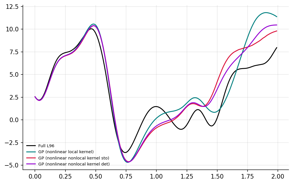
T_test = 10

X_full, _, _, _ = W.run(dt, T_test, return_coupling=True)  # Full model

init_cond = Xtrue[-1, :]

gcm_gp_nonlinear = GCM_GP(Forcing, gp_nonlinear, stochastic=True)
Xgp_nonlinear, t = gcm_gp_nonlinear(init_cond, dt, int(T_test / dt), gp_nonlinear)

gcm_gp_nonlocal = GCM_GP(Forcing, gp_nonlocal, stochastic=True, local=False)
Xgp_nonlocal, t = gcm_gp_nonlocal(init_cond, dt, int(T_test / dt), gp_nonlocal)

gcm_gp_nonlocal_det = GCM_GP(Forcing, gp_nonlocal, stochastic=False, local=False)
Xgp_nonlocal_det, t = gcm_gp_nonlocal_det(init_cond, dt, int(T_test / dt), gp_nonlocal)

time_i = 200
fig, ax = plt.subplots(1, figsize=(8, 5), dpi=150)
ax.spines["top"].set_color(None)
ax.spines["right"].set_color(None)
ax.plot(t[:time_i], X_full[:time_i, 4], label="Full L96", color="k")
ax.plot(
    t[:time_i],
    Xgp_nonlinear[:time_i, 4],
    label="GP (nonlinear local kernel)",
    color="teal",
)
ax.plot(
    t[:time_i],
    Xgp_nonlocal[:time_i, 4],
    label="GP (nonlinear nonlocal kernel sto)",
    color="crimson",
)
ax.plot(
    t[:time_i],
    Xgp_nonlocal_det[:time_i, 4],
    label="GP (nonlinear nonlocal kernel det)",
    color="darkviolet",
)
ax.grid(True, alpha=0.3)
plt.legend(frameon=False, fontsize=7)
plt.show()