Introduction to Machine Learning and Neural Networks#
Outline:#
In this notebook we introduce the basics of machine learning, show how to optimize parameters in simple models (linear regression), and finally demonstrate a basic neural network training case. There are many excellent tutorials on machine learning available on the internet, and our goal here is not to be comprehensive but rather provide a gentle introduction that seems necessary to what comes later in the book.
Introduction to machine learning#
Machine learning can be defined as : “Machine learning is a way for computers to learn and improve from experience without being explicitly programmed.” This definition was generated with the help of an AI agent called ChatGPT.
It has proven to be a useful tool to the scientific community by being able to make advancements in a range of problems, which had traditionally been very challenging or impossible. In our project, M2LInES, we are improving simulations of the climate system by targeting the parameterization or sub-grid closure problem with the help of ML.
In simpler terms, ML for our context can be thought of as a sophisticated way to approximate or estimate function. This can be done in a way where the structure of the functions is prescribed and constrained to very limited space of functions (e.g. linear regression) or in a way where the the structure of the function is left relatively free (e.g. neural networks). Regardless of this choice, all ML tasks can be broken down into a few general pieces:
Data : All ML tasks need data to learn patterns.
Model : Some choice needs to be made about the model architecture (e.g. neural network, gaussian process, etc).
Loss functions : The way a ML model gets closer to the true function is by minimizing some appropriately chosen loss function, a measure of error between truth and ML prediction.
Optimizers : To minize the error or loss function some method is needed to estimate optimal parameters.
Since all this is being done on a computer, some software architecture is needed. Possible, one of the major reasons for large scale adoption of machine learning has been the availability of easy to use, well documented, open source and general purpose machine learning libraries. Many such library exist, e.g. Tensorflow, PyTorch, JAX, etc. In this book we will primarily use PyTorch.
PyTorch#
In short, PyTorch is a Python-based machine learning framework that can be used for scientific machine learning tasks. There are many good reasons to use PyTorch, including that it can be used as a replacement for NumPy if we want to do computations on GPUs, it is extremely flexible and fast, but primarily that it has a large community and excellent tutorials to learn from.
To understand and install PyTorch, we recommend going through the tutorials, blogs, or one of the many online tutorial (e.g. Deep Learning With Pytorch: A 60 Minute Blitz, Neural Networks etc).
To follow along a single blogpost that goes through most concepts, we recommend this.
Having understood how the tools work, we can now use them to model our data. To train any machine learning model, there is a general recipe followed. This recipe can be summarized in three steps:
Define a model representation.
Choose a suitable loss function that tells us how far apart our model predictions are from the real data
Update the parameters in model representation using an optimization algorithm to minimize the loss function.
In this notebook, we will be working a linear regression model and a neural network. We will measure loss using the Mean Squared Error (MSE) function and will try to optimize or reduce the loss value using a popular optimization algorithm, gradient descent.
To read further on how to train machine learning models, refer to Prof. Fund’s lecture notes or Prof. Hegde’s blogposts.
Linear regression#
Probably, the simplest “machine learning” model is linear regression. This model models the relationship between the input and output data as a linear function, which for a single input and single output dimension is equivalent to fitting a line through the data: $\( y = w_1x + w_0, \)\( where \)w_1\( (slope or kernel) and \)w_0$ (bias) are parameters that need to best estimated.
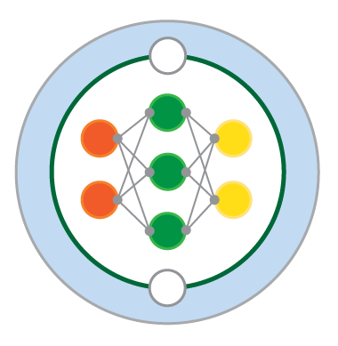
For multiple inputs and single output the model can be visually represented as follows:
Image is taken from here. Similarly, this linear regression could be modified to have multiple inputs and multiple outputs.
There are many ways to estimate optimal parameters for linear regression, and here we will show how this can be done using PyTorch and gradient descent.
The best prediction is defined by minimizing some cost or loss function. For linear regression, generally the mean sequare error between the expected output \(y\) and the prediction (\(\tilde{y}\)), defined as mean of \((y-\tilde{y})^2\) over all output dimensions and samples, is minimized.
Most of this lesson follows a tutorial from Jeremy Howard’s fast.ai lesson zero.
We will learn the parameters \(w_0\) and \(w_1\) of a line using PyTorch.
# Import machine-learning packages
import torch
from torch import nn

# Import plotting packages
from IPython.display import Image, HTML
from matplotlib.animation import FuncAnimation
import matplotlib.pyplot as plt
import time
import base64
import numpy as np

%matplotlib inline
Set random seed for reproducibility
np.random.seed(42)
Data generation for linear regression#
Since this is a toy problem, we first choose the true parameters so that we can later easily verify the success of our approach.
w = torch.as_tensor([3.0, 2])
w
# where 3 is the interesection point (sometimes also called bias) and 2 is the slope.
tensor([3., 2.])
Notice that we are using tensors here, which is a data structure used by PyTorch to easily deploy computations to CPUs or GPUs.
Then we create some data points x and y which are related to each other through the linear relationship and parameters chosen above.
# We create 100 data points.
n = 100
x = torch.ones(n, 2)

# uniformly sample x points between -1 and 1.
# Underscore functions in pytorch means replace the value (update)
x[:, 1].uniform_(-1.0, 1)

x[:6]
tensor([[ 1.0000, -0.3084],
        [ 1.0000,  0.7425],
        [ 1.0000, -0.7232],
        [ 1.0000, -0.0600],
        [ 1.0000, -0.6953],
        [ 1.0000, -0.0497]])
Note above that for each sample we have created two numbers. The first is 1, to be used with \(w_0\), and the second is x, to be used with \(w_1\).
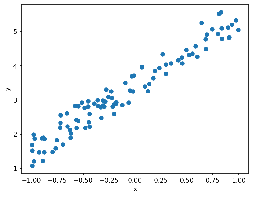
Next we generate output data using the equation for linear regression, but also add some random noise to be in the more real world setting where there is always some noise or if linear regression is not the perfect model.
# Generate output data.
y = x @ w + torch.rand(n)  # @ is a matrix product (similar to matmul)
plt.figure(dpi=150)
plt.scatter(x[:, 1], y)
plt.xlabel("x")
plt.ylabel("y")
plt.show();
Loss function#
We define our loss function \(L\) as Mean Square Error loss as:
def mse(y_true, y_pred):
    return ((y_true - y_pred) ** 2).mean()
Written in terms of \(w_0\) and \(w_1\), our loss function \(L\) is:
# Initialize parameters with some randomly guessed values.
w_real = torch.as_tensor([-3.0, -5])
y_hat = x @ w_real
# Initial mean-squared error
mse(y_hat, y)
tensor(48.1894)
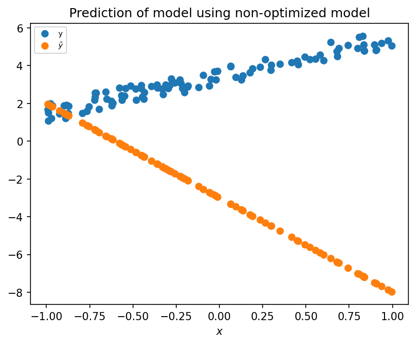
Here we chose randomly guessed initial parameter choices. While this choice is not consequential here, in more complex problems these choice prior parameter choice can be extremely important.
plt.figure(dpi=150)
plt.scatter(x[:, 1], y, label="y")
plt.scatter(x[:, 1], y_hat, label="$\\tilde{y}$")
plt.xlabel("$x$")
plt.title("Prediction of model using non-optimized model")
plt.legend(fontsize=7);
# Initialize parameter obect that will be optimized.
w = nn.Parameter(w_real)
w
Parameter containing:
tensor([-3., -5.], requires_grad=True)
Gradient descent and optimization#
So far, we have specified the model (linear regression) and the evaluation criteria (or loss function). Now we need to handle optimization; that is, how do we find the best values for weights (\(w_0\), \(w_1\)) such that they best fit the linear regression parameters?
This optimization is done using gradient descent. In this process the gradient of the loss function is estimated relative to the unknown parameters, and then the parameters are updated in a direction that reduces the loss function.
# Load the image file
with open("figs/Gradient_descent2.png", "rb") as f:
    image_data = f.read()

# Create the HTML code to display the image
html = f'<div style="text-align:center"><img src="data:image/png;base64,{base64.b64encode(image_data).decode()}" style="max-width:700px;"/></div>'

# Display the HTML code in the notebook
display(HTML(html))

To know how to change \(w_0\) and \(w_1\) to reduce the loss, we compute the derivatives (or gradients):
Since we know that we can iteratively take little steps down along the gradient to reduce the loss, aka, gradient descent, the size of the step is determined by the learning rate (\(\eta\)):
The gradients needed above are computed using the ML library’s autograd feature, and described more here.
def step(lr):
    y_hat = x @ w
    loss = mse(y, y_hat)
    # calculate the gradient of a tensor! It is now stored at w.grad
    loss.backward()

    # To prevent tracking history and using memory
    # (code block where we don't need to track the gradients but only modify the values of tensors)
    with torch.no_grad():
        # lr is the learning rate. Good learning rate is a key part of Neural Networks.
        w.sub_(lr * w.grad)
        # We want to zero the gradient before we are re-evaluate it.
        w.grad.zero_()

    return loss.detach().item(), y_hat.detach().numpy()
Note: In PyTorch, we need to set the gradients to zero before starting to do back propragation because PyTorch accumulates the gradients on subsequent backward passes. This is convenient while training Recurrent Neural Networks (RNNs). So, the default action is to accumulate or sum the gradients on every
loss.backward()call. Because of this, when you start your training loop, ideally you should zero out the gradients so that you do the parameter update correctly. Else the gradient would point in some other direction than the intended direction towards the minimum (or maximum, in case of maximization objectives).
w = torch.as_tensor([-2.0, -3])
w = nn.Parameter(w)
lr = 0.1
losses = [float("inf")]
y_hats = []
epoch = 100
# Train model and perform gradient descent
for _ in range(epoch):
    loss, y_hat = step(lr)
    losses.append(loss)
    y_hats.append(y_hat)
plt.figure(dpi=150)
plt.plot(np.array(losses))
plt.xlabel("Iteration")
plt.ylabel("Loss")
plt.yscale("log")
plt.title("Loss vs Iteration")
plt.show();
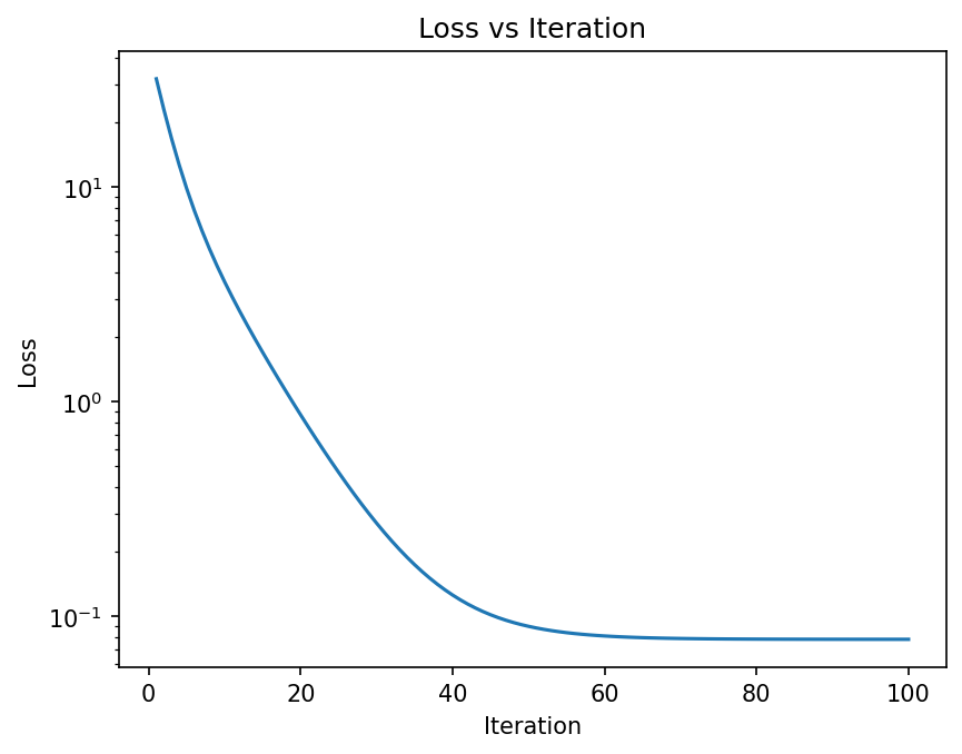
As seen above the loss function is reduced as more optimization steps are taken. The animation below shows how the prediction gets closer to the data as more steps are taken.
fig, axs = plt.subplots(1, 2, figsize=(10, 4), dpi=80)
axs[0].scatter(x[:, 1], y, label="y")
scatter_yhat = axs[0].scatter(x[:, 1], y_hat, label="$\\tilde{y}$")
axs[0].set_xlabel("$x$")
axs[0].legend(fontsize=7)

(line,) = axs[1].plot(range(len(losses)), np.array(losses))
axs[1].set_xlabel("Iteration")
axs[1].set_ylabel("Loss")
axs[1].set_title("Loss vs Iteration")
plt.close()


def animate(i):
    axs[0].set_title("Loss = %.2f" % losses[i])
    scatter_yhat.set_offsets(np.c_[[], []])
    scatter_yhat.set_offsets(np.c_[x[:, 1], y_hats[i]])
    line.set_data(np.array(range(i + 1)), np.array(losses[: (i + 1)]))
    return scatter_yhat, line


# plt.show()

animation = FuncAnimation(fig, animate, frames=epoch, interval=100, blit=True)
# let animation load
time.sleep(1)
plt.show();
In case you have some difficulties running the cell below without importing certain packages. Run the following code in a terminal in L96M2lines environment.
conda install -c conda-forge ffmpeg
display(HTML(f'<div style="text-align:center;">{animation.to_html5_video()}</div>'))
Neural Networks#
The above discussion focussed on fitting a simple function, a line, through our data. However, data in many problems correspond to underlying functions that are much more complex and their exact form is not known. For these problem we need functions that are much more flexible; neural networks are these more flexible functions.
This is shown by the Universal Approximation Theorm, which states that neural networks can approximate any continuous function. A visual demonstration that neural nets can compute any function can be seen in this page.
Now we give a brief overview of neural networks and how to build them using PyTorch. If you want to go through it in depth, check out these resources: Deep Learning With Pytorch: A 60 Minute Blitz or Neural Networks.
Generate some data#
# We create many data points, as neural networks need lot of data to train from scratch.
n = 10000
x = torch.ones(n, 1)
# uniformly sample x points between -1 and 1.
# Underscore functions in pytorch means replace the value (update)
x = x.uniform_(-1.0, 1)
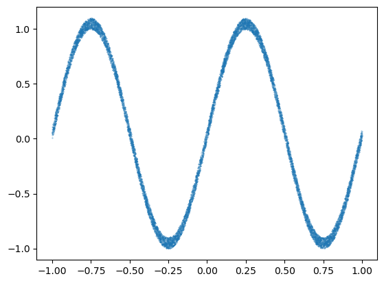
y = torch.sin(x * 2 * torch.pi) + 0.1 * torch.rand(n, 1)
In this problem we create a more wigly function (sin), which can not be approximated as a line.
plt.plot(x[:, 0], y, ".", markersize=0.5)
[<matplotlib.lines.Line2D at 0x7f6539425ee0>]
Define the neural network#
There are many many flavors of neural networks, as can be seen at the neural network zoo. Here we use the simplest - a fully connected neural net.
Visually the fully connected neural networks may be represented as:

Fig. 2 A neural network with 4 hidden layers and an output layer.#
Our particular design consists of 3 hidden dense layers, two of which have a non-linear Relu activation function.
class Simple_Neural_Net(nn.Module):
    def __init__(self):
        super().__init__()
        self.Dense1 = nn.Linear(1, 30)
        self.Dense2 = nn.Linear(30, 30)
        self.Dense3 = nn.Linear(30, 1)

        self.relu = nn.ReLU()

    def forward(self, x):
        # This method is automatically executed when
        # we call a object of this class
        x = self.Dense1(x)
        x = self.relu(x)
        x = self.Dense2(x)
        x = self.relu(x)
        x = self.Dense3(x)

        return x
neural_net = Simple_Neural_Net()
net_input = torch.randn(1, 1)
out = neural_net(net_input)
print(
    f"The output of the random input {net_input.item():.4f} from untrained network is: {out.item():.4f}"
)
The output of the random input -0.7623 from untrained network is: -0.1678
Updating the Weights using an Optimizer#
In the linear regression problem above we used a very simple optimization procedure, just adjusting the weights manually. However, in more complex problems it is sometimes more convenient to use the optimization module available in PyTorch as it can allow the use of many advanced options. The implementation of almost every optimizer that we’ll ever need can be found in PyTorch itself. The choice of which optimizer we choose might be very important as it will determine how fast the network will be able to learn.
In the example below, we show one of the popular optimizers Adam.
Adam Optimizer#
A popular optimizer that is used in many neural networks is the Adam optimizer. It is an adaptive learning rate method that computes individual learning rates for different parameters. For further reading, check out this post about Adam, and this post about other optimizers.
# Here we use the Adam optimizer.
learning_rate = 0.005
optimizer = torch.optim.Adam(neural_net.parameters())
Loss function#
We use the mean square error as loss function again.
# MSE loss function
loss_fn = torch.nn.MSELoss()
Training the network#
The training step is defined below, where optimizer.step() essentially does the job of updating the parameters.
def train_step(model, loss_fn, optimizer):
    # Set the model to training mode - important for batch normalization and dropout layers
    # Unnecessary in this situation but added for best practices

    pred = model(x)
    loss = loss_fn(pred, y)

    # Backpropagation
    loss.backward()
    optimizer.step()
    optimizer.zero_grad()

    loss = loss.item()
    return loss
When it comes to real training problems, often the data sets are very large and can not be fit into memory. In these cases the data might be broken up into smaller chunks called batches, and the training is done on one batch at a time. A pass over all the batches in the data set is referred to as an epoch. Since our data set is very small we do not break it up into batches here, but still refer to each training step as an epoch.
epochs = 1000
Loss = np.zeros(epochs)
for t in range(epochs):
    Loss[t] = train_step(neural_net, loss_fn, optimizer)
    if np.mod(t, 200) == 0:
        print(f"Loss at Epoch {t+1} is ", Loss[t])
Loss at Epoch 1 is  0.5483013391494751
Loss at Epoch 201 is  0.1875164657831192
Loss at Epoch 401 is  0.055956799536943436
Loss at Epoch 601 is  0.0175771564245224
Loss at Epoch 801 is  0.00432428577914834
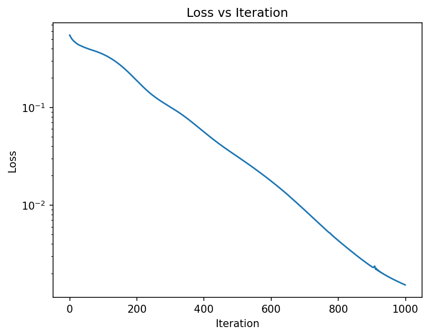
plt.figure(dpi=150)
plt.plot(Loss)
plt.xlabel("Iteration")
plt.ylabel("Loss")
plt.yscale("log")
plt.title("Loss vs Iteration")
plt.show();
Compare Predictions with Ground Truth#
# Generate some points where the predictions of the model will be tested.
# Here we pick the testing domain to be larger than the training domain to check if the model
# has any skill at extrapolation.
x_test = torch.linspace(-1.5, 1.5, 501).reshape(501, 1)

# Generate the predictions from the trained model.
pred = neural_net(x_test).detach().numpy()
plt.figure(dpi=150)

plt.plot(x, y, ".", markersize=0.5, label="Data")
plt.plot(x_test, pred, markersize=0.5, label="Predicted fit")

plt.legend()
<matplotlib.legend.Legend at 0x7f651a853a00>
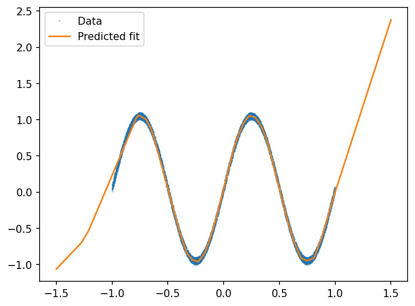
As seen above, the neural network is able to approximate the sine function relatively well over the range over which the training data is available. However, it should also be noted that the neural network possesses no skill to extrapolate beyond the range of the data that it was trained on.
Summary#
In this notebook we introduced the basics of machine learning - fitting flexible functions to data. In the next few notebooks we will show how neural networks can be used to model sub-grid forcing in the Lorenz 96 model, and also some more useful topics related to neural network training and interpretation.