Introduction to Equation Discovery - Comparing Symbolic Regression Methods#
Upto now we have seen that the climate models we developed are using physical equations that are based on our understanding of the physical processes that govern the climate. However, these equations are often complex and difficult to solve, and they can only be used to model the climate at a coarse resolution.
Equation discovery is a different approach that uses machine learning to automatically discover equations that can be used to model the climate. Specifically, equation discovery in climate modeling can be used to:
Automate the process of developing subgrid parameterizations. Subgrid parameterizations are mathematical equations that are used to represent the effects of processes that are too small to be resolved by climate models. These equations are often complex and difficult to develop, but they can be automatically discovered using equation discovery.
Identify relationships between variables that are important for understanding climate change. Machine learning algorithms can learn from large datasets of climate data to identify relationships between variables that are important for understanding climate change.
Develop models that are more interpretable and that can be used to make better decisions about how to mitigate and adapt to climate change. Machine learning algorithms can generate equations that are easier to understand than traditional physical equations. This can help scientists and policymakers to understand how climate models work and to make better decisions about how to mitigate and adapt to climate change.
In this notebook, we’ll review some common techniques for Symbolic Regression (SR), a family of methods of discovering (simple) equations that relate inputs to outputs.
In particular, we’ll cover the following methods:
Symbolic regression based on Genetic Programming
Symbolic regression based on Manually Constructed Library + Sparse Regression
Brief overview of other techniques
%matplotlib inline
import matplotlib.pyplot as plt
import numpy as np
import pysindy as ps
from sklearn.linear_model import Lasso, LinearRegression
from sympy import Number, latex

from rvm import RVR
Data#
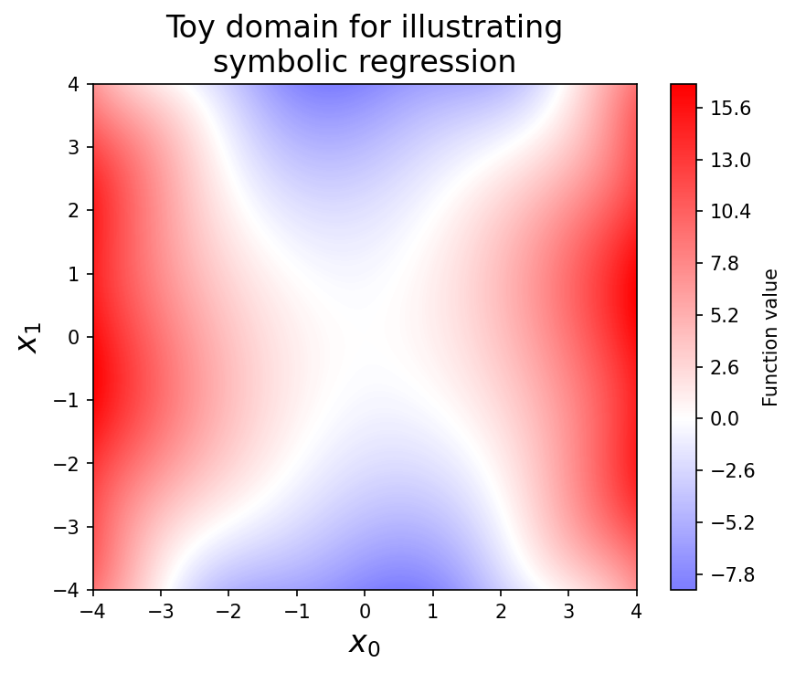
When explaining the methods, we’ll consider the following bivariate system:
Although the equation is relatively simple, discovering it from \(x_0\) and \(x_1\) directly is a bit tough, since the \(\sin\) term requires going at least three levels deep in term combinations, and also involves an inner multiplication by a constant (which not all symbolic regression frameworks support).
def toy_function(x):
    x0 = x[:, 0]
    x1 = x[:, 1]
    return x0**2 - 0.5 * x1**2 + np.sin(0.5 * x0 * x1)
def contour(
    f, lines=None, linewidths=6, alpha=0.9, linestyles="solid", label=None, **kw
):
    grid = np.linspace(-4, 4, 150)
    xyg = np.array(np.meshgrid(grid, grid))
    X = xyg.reshape(2, -1).T
    zg = f(X)
    xg, yg = xyg
    vlim = np.abs(zg).max()
    plt.contourf(xg, yg, zg.reshape(xg.shape), 300, vmin=-vlim, vmax=vlim, cmap="bwr")
    plt.colorbar(label=label)
x = np.random.normal(size=(1000, 2))
y = toy_function(x)
plt.figure(dpi=150)
contour(toy_function, label="Function value")
plt.title("Toy domain for illustrating\nsymbolic regression", fontsize=16)
plt.xlabel("$x_0$", fontsize=16)
plt.ylabel("$x_1$", fontsize=16)
plt.show()
Genetic Programming#
Genetic programming is a classic technique in AI, and interest in the idea dates back at least to Alan Turing (who proposes the idea in the same paper that introduces the imitation game, or Turing test).
The general idea is to have a:
“Population” of programs (in our case, possible symbolic expressions, usually represented as trees)
Some notion of individual “fitness” (in our case, how well they model the data, as well as their simplicity)
Some means of applying random “mutations” (e.g. adding a term, deleting a term)
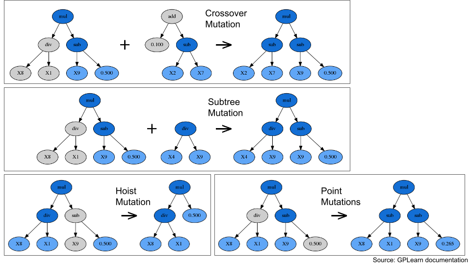
Fig. 6 Some examples for different mutation types#
“Crossover” and “subtree” mutations combine features from multiple candidate equations, imitating the process of genetic recombination from sexual reproduction. “Hoist” and “point” mutations modify individual equations, imitating the process of genetic mutation from, e.g., random errors in DNA replication.
Specific mutations aside, programs can have a limited lifespan, and those with high “fitness” produce more “offspring” (possibly-mutated versions of themselves). However, everything is probabilistic, so programs with lower fitness can still persist. This is critically important, because it allows genetic programming to overcome local minima during optimization.
Note that although genetic programming can be a robust way to solve extremely difficult non-convex optimization problems (as perhaps evidenced by life itself), it also tends to be slow and resource-intensive.
gplearn#
One nicely-documented library for “pure” genetic programming-based symbolic regression is gplearn, which provides a scikit-learn style API and a number of configuration options:
Run gplearn#
import gplearn
import gplearn.genetic
gplearn_sr = gplearn.genetic.SymbolicRegressor(
    population_size=5000,
    generations=50,
    p_crossover=0.7,
    p_subtree_mutation=0.1,
    p_hoist_mutation=0.05,
    p_point_mutation=0.1,
    max_samples=0.9,
    verbose=1,
    parsimony_coefficient=0.01,
    function_set=("add", "mul", "sin"),
)
gplearn_sr.fit(x, y)
    |   Population Average    |             Best Individual              |
---- ------------------------- ------------------------------------------ ----------
 Gen   Length          Fitness   Length          Fitness      OOB Fitness  Time Left
   0    18.27          1.51607       63         0.484344         0.506384      2.30m
   1     7.03          1.01195       12         0.500263         0.352436      1.82m
   2     6.22         0.942033        9        0.0859325         0.072056      1.67m
   3     3.64         0.815446        9        0.0835414        0.0935763      1.56m
   4     3.66         0.807118        9        0.0802486         0.123211      1.49m
   5     4.65         0.871852        9        0.0586539        0.0483341      1.48m
   6     7.73         0.937853        9        0.0556039        0.0757836      1.58m
   7     8.99         0.952487        9        0.0513895         0.113714      1.55m
   8     9.12         0.945486        9        0.0491828         0.133574      1.48m
   9     8.95           0.9445        9        0.0481976         0.142441      1.48m
  10     8.88         0.949946        9        0.0450134        0.0196311      1.40m
  11     8.86         0.939362        9         0.039291        0.0711325      1.36m
  12     8.99         0.965802        9        0.0379511        0.0831918      1.37m
  13     9.02         0.948019        9        0.0361227        0.0996473      1.29m
  14     9.06         0.933539        9        0.0348376         0.111213      1.25m
  15     9.01         0.940116        9        0.0333682         0.124438      1.25m
  16     9.01         0.945087        9        0.0334012         0.124141      1.18m
  17     9.04         0.949223        9        0.0331261         0.126617      1.15m
  18     9.01         0.957547        9        0.0327036         0.130419      1.16m
  19     9.06         0.945616        9        0.0345203         0.114069      1.08m
  20     9.03          0.94679        9        0.0322441         0.134555      1.04m
  21     9.05         0.928582        9        0.0340354         0.118433      1.04m
  22     9.07         0.953325        9         0.032703         0.130425     58.08s
  23     8.94         0.945337        9        0.0329236         0.128439     55.86s
  24     8.95         0.949259        9        0.0339025         0.119629     53.84s
  25     9.01         0.961325        9        0.0340025         0.118729     54.24s
  26     8.98         0.945117        9        0.0335818         0.122516     49.60s
  27     9.09         0.927206        9        0.0334483         0.123717     47.56s
  28     8.97         0.948439        9        0.0324886         0.132355     46.92s
  29     8.95         0.945998        9        0.0337105         0.121357     43.26s
  30     9.04         0.948537        9        0.0332377         0.125613     41.03s
  31     8.98          0.95871        9        0.0338695         0.119926     40.53s
  32     8.99         0.962767        9        0.0339732         0.118993     36.94s
  33     9.05          0.93255        9        0.0330054         0.127703     36.11s
  34     9.17          0.94233        9        0.0332547         0.125459     32.71s
  35     8.98         0.959933        9        0.0343294         0.115788     30.41s
  36     9.06         0.957752        9        0.0338502           0.1201     28.21s
  37     9.05         0.928806        9        0.0333783         0.124347     27.16s
  38     8.99         0.952908        9        0.0340984         0.117866     23.89s
  39     9.12         0.947681        9         0.034453         0.114675     21.76s
  40     9.03         0.934268        9           0.0339         0.119652     20.42s
  41     9.02         0.944012        9        0.0342319         0.116665     17.46s
  42     8.90         0.934928        9         0.034021         0.118563     15.29s
  43     8.94         0.929862        9        0.0348036          0.11152     13.71s
  44     9.08         0.962178        9        0.0326351         0.131036     10.94s
  45     9.03         0.942342        9        0.0346503         0.112899      8.78s
  46     9.03         0.932699        9        0.0346973         0.112476      6.88s
  47     9.02         0.929394        9        0.0335859         0.122479      4.37s
  48     8.96         0.942558        9        0.0330422         0.127372      2.21s
  49     9.00         0.931138        9         0.034178          0.11715      0.00s
mul(add(X1, X0), add(X0, mul(X1, -0.499)))In a Jupyter environment, please rerun this cell to show the HTML representation or trust the notebook.
On GitHub, the HTML representation is unable to render, please try loading this page with nbviewer.org.
mul(add(X1, X0), add(X0, mul(X1, -0.499)))
Interpret results#
print(gplearn_sr._program)
mul(add(X1, X0), add(X0, mul(X1, -0.499)))
This looks very close to the right answer, though the constants are slightly off.
[const for const in gplearn_sr._program.program if isinstance(const, float)]
[-0.4990643478749499]
This is likely because gplearn mutations which add or update constants always pick values by drawing random uniform values (within pre-specified ranges, by default -1 to 1). In my limited experience so far, this is one of the major inefficiencies.
PySR#
PySR is a different library for symbolic regression which, though still based on genetic programming, includes simulated annealing and gradient-free optimization to set the values of constants as well as performance improvements (although accessible via a Python API, the main library is written in Julia for speed). This seems to make it a bit more reliable and precise.
Run PySR#
import pysr
equations = pysr.PySRRegressor(
    niterations=5,
    binary_operators=["+", "*"],  # operators that can combine two terms
    unary_operators=["sin"],  # operators that modify a single term
)
equations.fit(x, y)
Compiling Julia backend...
Started!
PySRRegressor.equations_ = [
	    pick         score                                           equation  \
	0         0.000000e+00                                         0.45667043
	1         5.373556e-01                                          (x0 * x0)
	2         1.533802e-01                          ((x0 * x0) + -0.49401912)
	3         1.470930e-07                     ((x0 * x0) + sin(-0.51677376))
	4         1.552197e-03              (((x0 + 0.03341666) * x0) + -0.49697)
	5         1.009282e-01               (((sin(x1) + x0) * x0) + -0.4792763)
	6         2.764493e+00            ((x0 + (x1 * -0.53268653)) * (x0 + x1))
	7         2.512280e-03  ((x0 + ((x1 * 0.97228694) * -0.53268653)) * (x...
	8         2.959594e-01  (((x0 + (0.4008724 * x1)) * x0) + ((-0.4881864...
	9   >>>>  4.450350e-01  (((x0 + (sin(x1) * 0.5425623)) * x0) + ((-0.48...
	10        1.542535e-02  (((x0 + sin(sin(sin(x1 * 0.5425623)))) * x0) +...
	11        1.174728e-01  (((x0 + sin(sin(sin(sin(x1 * 0.5425623))))) * ...

	        loss  complexity
	0   2.706285           1
	1   0.923916           3
	2   0.679842           5
	3   0.679842           6
	4   0.678787           7
	5   0.613622           8
	6   0.038663           9
	7   0.038469          11
	8   0.021284          13
	9   0.013639          14
	10  0.013224          16
	11  0.011759          17
]
In a Jupyter environment, please rerun this cell to show the HTML representation or trust the notebook.
On GitHub, the HTML representation is unable to render, please try loading this page with nbviewer.org.
PySRRegressor.equations_ = [
	    pick         score                                           equation  \
	0         0.000000e+00                                         0.45667043
	1         5.373556e-01                                          (x0 * x0)
	2         1.533802e-01                          ((x0 * x0) + -0.49401912)
	3         1.470930e-07                     ((x0 * x0) + sin(-0.51677376))
	4         1.552197e-03              (((x0 + 0.03341666) * x0) + -0.49697)
	5         1.009282e-01               (((sin(x1) + x0) * x0) + -0.4792763)
	6         2.764493e+00            ((x0 + (x1 * -0.53268653)) * (x0 + x1))
	7         2.512280e-03  ((x0 + ((x1 * 0.97228694) * -0.53268653)) * (x...
	8         2.959594e-01  (((x0 + (0.4008724 * x1)) * x0) + ((-0.4881864...
	9   >>>>  4.450350e-01  (((x0 + (sin(x1) * 0.5425623)) * x0) + ((-0.48...
	10        1.542535e-02  (((x0 + sin(sin(sin(x1 * 0.5425623)))) * x0) +...
	11        1.174728e-01  (((x0 + sin(sin(sin(sin(x1 * 0.5425623))))) * ...

	        loss  complexity
	0   2.706285           1
	1   0.923916           3
	2   0.679842           5
	3   0.679842           6
	4   0.678787           7
	5   0.613622           8
	6   0.038663           9
	7   0.038469          11
	8   0.021284          13
	9   0.013639          14
	10  0.013224          16
	11  0.011759          17
]
Interpret results#
def round_expr(expr, num_digits=4):
    return expr.xreplace({n: round(n, num_digits) for n in expr.atoms(Number)})
round_expr(equations.sympy())
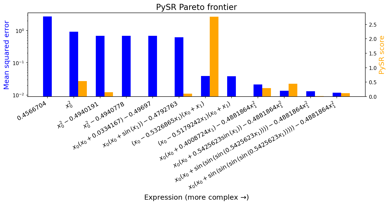
It looks like PySR is able to not only discover the correct equation, but also format it for us nicely.
In addition, it saves a Pareto frontier of possible expressions of varying complexities, which had the lowest error of any other equations of equal or lesser complexity (with a configurable trade-off rule):
equations.equations_
| complexity | loss | score | equation | sympy_format | lambda_format | |
|---|---|---|---|---|---|---|
| 0 | 1 | 2.706285 | 0.000000e+00 | 0.45667043 | 0.456670430000000 | PySRFunction(X=>0.456670430000000) |
| 1 | 3 | 0.923916 | 5.373556e-01 | (x0 * x0) | x0**2 | PySRFunction(X=>x0**2) |
| 2 | 5 | 0.679842 | 1.533802e-01 | ((x0 * x0) + -0.49401912) | x0**2 - 0.49401912 | PySRFunction(X=>x0**2 - 0.49401912) |
| 3 | 6 | 0.679842 | 1.470930e-07 | ((x0 * x0) + sin(-0.51677376)) | x0**2 - 0.494077763833335 | PySRFunction(X=>x0**2 - 0.494077763833335) |
| 4 | 7 | 0.678787 | 1.552197e-03 | (((x0 + 0.03341666) * x0) + -0.49697) | x0*(x0 + 0.03341666) - 0.49697 | PySRFunction(X=>x0*(x0 + 0.03341666) - 0.49697) |
| 5 | 8 | 0.613622 | 1.009282e-01 | (((sin(x1) + x0) * x0) + -0.4792763) | x0*(x0 + sin(x1)) - 0.4792763 | PySRFunction(X=>x0*(x0 + sin(x1)) - 0.4792763) |
| 6 | 9 | 0.038663 | 2.764493e+00 | ((x0 + (x1 * -0.53268653)) * (x0 + x1)) | (x0 - 0.53268653*x1)*(x0 + x1) | PySRFunction(X=>(x0 - 0.53268653*x1)*(x0 + x1)) |
| 7 | 11 | 0.038469 | 2.512280e-03 | ((x0 + ((x1 * 0.97228694) * -0.53268653)) * (x... | (x0 - 0.517924156232918*x1)*(x0 + x1) | PySRFunction(X=>(x0 - 0.517924156232918*x1)*(x... |
| 8 | 13 | 0.021284 | 2.959594e-01 | (((x0 + (0.4008724 * x1)) * x0) + ((-0.4881864... | x0*(x0 + 0.4008724*x1) - 0.48818642*x1**2 | PySRFunction(X=>x0*(x0 + 0.4008724*x1) - 0.488... |
| 9 | 14 | 0.013639 | 4.450350e-01 | (((x0 + (sin(x1) * 0.5425623)) * x0) + ((-0.48... | x0*(x0 + 0.5425623*sin(x1)) - 0.48818642*x1**2 | PySRFunction(X=>x0*(x0 + 0.5425623*sin(x1)) - ... |
| 10 | 16 | 0.013224 | 1.542535e-02 | (((x0 + sin(sin(sin(x1 * 0.5425623)))) * x0) +... | x0*(x0 + sin(sin(sin(0.5425623*x1)))) - 0.4881... | PySRFunction(X=>x0*(x0 + sin(sin(sin(0.5425623... |
| 11 | 17 | 0.011759 | 1.174728e-01 | (((x0 + sin(sin(sin(sin(x1 * 0.5425623))))) * ... | x0*(x0 + sin(sin(sin(sin(0.5425623*x1))))) - 0... | PySRFunction(X=>x0*(x0 + sin(sin(sin(sin(0.542... |
equations.equations_.loss
0     2.706285
1     0.923916
2     0.679842
3     0.679842
4     0.678787
5     0.613622
6     0.038663
7     0.038469
8     0.021284
9     0.013639
10    0.013224
11    0.011759
Name: loss, dtype: float64
plt.figure(figsize=(12, 3), dpi=150)
plt.bar(
    np.arange(len(equations.equations_)),
    equations.equations_.loss,
    width=0.33,
    color="blue",
)


plt.yscale("log")
plt.ylabel("Mean squared error", fontsize=14, color="blue")
plt.xticks(
    range(len(equations.equations_)),
    [f"${latex(round_expr(v,7))}$" for v in equations.equations_.sympy_format],
    rotation=30,
    ha="right",
    fontsize=12,
)
plt.title("PySR Pareto frontier", fontsize=16)
plt.xlabel("Expression (more complex $\\to$)", fontsize=14)

ax2 = plt.twinx()
ax2.bar(
    np.arange(len(equations.equations_)) + 0.33,
    equations.equations_.score,
    width=0.33,
    color="orange",
)
ax2.set_ylabel("PySR score", color="orange", fontsize=14)

plt.show()
Manually Constructed Library + Sparse Regression#
Another approach to performing symbolic regression is to
Hand-construct a library of basis functions (e.g. by recursively combining all terms with various operations)
Run sparse linear regression to extract a small set of basis functions
This approach works well for problems where any constants in the underlying formula can be extracted out to the outermost level (so they can be determined by linear regression). It also works well when we have domain knowledge about which terms could potentially appear in the final sum.
It does not work well in cases where constants can’t be pulled outside certain operations (e.g. in this case, with the sine operator, though powers and derivatives are generally fine). This method can also struggle when basis function values are highly correlated, though it depends on the sparse regression method.
Let’s create an augmentation function which takes an array of features and adds additional basis functions by combining them with binary multiplication and unary sine operations:
def augment(feats, names):
    existing = set(names)
    new_feats = []
    new_names = []

    for i in range(feats.shape[1]):
        name = f"sin({names[i]})"
        if name not in existing:
            new_feats.append(np.sin(feats[:, i]))
            new_names.append(name)
        for j in range(i, feats.shape[1]):
            name = f"mul({names[i]}, {names[j]})"
            if name not in existing:
                new_feats.append(feats[:, i] * feats[:, j])
                new_names.append(name)

    return np.hstack((feats, np.array(new_feats).T)), names + new_names
def repeatedly_augment(feats, names=None, depth=2):
    if names is None:
        names = [f"x{i}" for i in range(len(feats))]
    for _ in range(depth):
        feats, names = augment(feats, names)
    return feats, names
feats, names = repeatedly_augment(np.array(x), ["x0", "x1"], depth=2)
Applying this twice brings us from 2 features up to 37:
feats.shape
(1000, 37)
We can see that the complexity of this approach starts to blow up exponentially, though, as we increase the maximum depth of an expression:
augment(feats, names)[0].shape
(1000, 742)
augment(*augment(feats, names))[0].shape
(1000, 276397)
If we need arbitrary polynomials of up to 4th order, we end up with orders of magnitude more features than samples, which will cause problems.
Note that since this method lacks the ability to apply operations with constants within other operations, \(\sin(0.5 x_0 x_1)\) isn’t present in any of these possible sets, though \(\sin(x_0 x_1)\) is.
Let’s now see how different methods for (sparse) linear regression perform on this task:
def learned_expr(coef, names, cutoff=1e-2):
    coef_idx = np.argwhere(np.abs(coef) > cutoff)[:, 0]
    sort_order = reversed(np.argsort(np.abs(coef[coef_idx])))
    return " + ".join(
        [f"{coef[coef_idx[i]]:.4f}*{names[coef_idx[i]]}" for i in sort_order]
    )
Linear regression#
We can start with completely unregularized linear regression, which will find the linear combination of basis terms that minimizes mean squared error (to high precision, due to the convexity of the problem and an analytic way of solving it).
linreg = LinearRegression()
linreg.fit(feats, y)
learned_expr(linreg.coef_, names)
'0.9926*mul(x0, x0) + -0.8851*mul(sin(x0), sin(x1)) + 0.8132*mul(x0, sin(x1)) + 0.7523*mul(x1, sin(x0)) + -0.4504*mul(x1, x1) + -0.2790*x1 + -0.2487*x0 + 0.2277*sin(x1) + 0.2176*sin(x0) + -0.2019*mul(x0, x1) + -0.0836*mul(x1, sin(x1)) + 0.0505*sin(sin(x1)) + 0.0395*mul(sin(x1), sin(x1)) + 0.0326*sin(sin(x0)) + 0.0279*mul(x1, mul(x1, x1)) + 0.0255*mul(x0, mul(x0, x0)) + 0.0247*mul(sin(x1), mul(x1, x1)) + 0.0194*mul(sin(x0), mul(x0, x0)) + 0.0179*sin(mul(x0, x1)) + -0.0160*mul(mul(x0, x0), mul(x0, x1)) + 0.0129*mul(x0, sin(x0))'
Unfortunately, this doesn’t seem to give us a very sparse solution in this case.
L1-regularized linear regression (LASSO)#
A common way to make linear regression return more sparse solutions is to minimize a linear combination of the mean squared error and the sum of the magnitudes of the weights. This is called applying an “L1 penalty” since it is the L1-norm of the weight vector, and is also referred to as the “Least Absolute Shrinkage and Selection Operator”, or LASSO. From a Bayesian perspective, this corresponds to doing Bayesian linear regression with a Laplace or double-exponential prior on the weights.
Note that although this penalty does tend to encourage sparsity, it’s also meant as a regularizer, which can help with the presence of noise.
lasso = Lasso(alpha=0.01)
lasso.fit(feats, y)
learned_expr(lasso.coef_, names)
'0.9757*mul(x0, x0) + -0.4868*mul(x1, x1) + 0.2800*mul(x0, x1) + 0.1723*mul(x1, sin(x0)) + 0.0948*sin(mul(x0, x1)) + -0.0251*mul(mul(x0, x1), mul(x1, x1))'
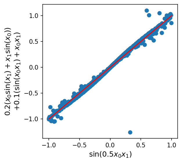
Here, LASSO ends up doing a pretty good job finding the first two terms of the ground-truth model (\(x_0^2 - 0.5x_1^2\)), with an approximation of the remaining \(\sin(0.5 x_0 x_1)\) term as \( 0.2(x_0\sin(x_1)+x_1\sin(x_0)) + 0.1(\sin(x_0 x_1) + x_0x_1)\):
plt.figure(figsize=(4, 4), dpi=150)
x0 = x[:, 0]
x1 = x[:, 1]
sin = np.sin
plt.scatter(
    sin(0.5 * x0 * x1),
    0.2 * (x0 * sin(x1) + x1 * sin(x0)) + 0.1 * (sin(x0 * x1) + x0 * x1),
)
plt.plot([-1, 1], [-1, 1], color="red")
plt.xlabel(r"$\sin(0.5 x_0 x_1)$", fontsize=12)
plt.ylabel(
    r"$0.2(x_0\sin(x_1)+x_1\sin(x_0))$" + "\n" + r"$+ 0.1(\sin(x_0 x_1) + x_0x_1)$",
    fontsize=12,
)
plt.show()
Relevance vector machines (RVM)#
Relevance vector machines, used by Zanna and Bolton 2020 for equation discovery, provide another way of learning sparse linear models in a Bayesian manner, though with a different prior that prioritizes sparsity over shrinkage when the data permits it. RVMs can also be used with a kernel trick to learn nonlinear decision boundaries which are sparse in a kernelized feature space, though in this case, we use a linear kernel on top of our manually computed library features.
rvm = RVR(verbose=False)
rvm.fit(feats, y, names)
learned_expr(rvm.m_, rvm.labels)
'0.9635*mul(x0, x0) + -0.8821*mul(sin(x0), sin(x1)) + 0.7994*mul(x0, sin(x1)) + 0.7523*mul(x1, sin(x0)) + -0.4860*mul(x1, x1) + -0.1941*mul(x0, x1) + 0.0617*mul(x0, sin(x0)) + -0.0297*mul(sin(x0), sin(x0)) + -0.0230*mul(x1, sin(x1)) + 0.0204*sin(mul(x0, x1)) + -0.0153*mul(mul(x0, x0), mul(x0, x1)) + 0.0150*sin(x0) + -0.0146*sin(sin(x0)) + -0.0115*sin(sin(x1)) + 0.0102*mul(sin(x1), sin(x1))'
RVM does discover the \(x_0^2\) and \(-0.5x_1^2\) terms almost exactly, but ends up with an even more complex approximate expression for the missing \(\sin(0.5x_0x_1)\) term.
Sequentially Thresholded Least Squares (STLSQ) from pysindy#
The PySINDy library provides a number of efficient Python implementations of sparse regression algorithms. Their default regression method is sequentially thresholded least squares (STLSQ), which (as its name might suggest) repeatedly runs L2-regularized linear regression with penalty strength alpha and prunes features with weight magnitudes below a given threshold.
stlsq = ps.optimizers.stlsq.STLSQ(alpha=0.0001, threshold=0.1)
stlsq.fit(feats, y)
learned_expr(stlsq.coef_[0], names)
'0.9992*mul(x0, x0) + 0.8822*mul(x1, sin(x0)) + 0.8627*mul(x0, sin(x1)) + -0.8247*mul(sin(x0), sin(x1)) + -0.4996*mul(x1, x1) + -0.4000*mul(x0, x1)'
This method ends up finding a sparser solution than Lasso, though I did tweak the parameters a bit to make that happen :)
It’s worth checking out PySINDy’s full suite of sparse regression methods for other approaches!
Overall, all of these methods were able to find the \(x_0^2\) and \(-0.5x_1^2\) terms, but all of them also needed to find approximations for the remaining term because it wasn’t in the feature library. Meaning the expressions are both less accurate and more complex.
Tweaking the Feature Library#
Now, we can potentially resolve some of these issues by pre-multiplying \(x_1\) by 0.5 before the augmentation process (which we’ll call \(x_{1h}\)).
feats2 = np.array(x)
feats2[:, 1] = feats2[:, 1] * 0.5
names2 = ["x0", "x1h"]
depth = 2

for _ in range(depth):
    feats2, names2 = augment(feats2, names2)
In this case, the correct model should be expressed as
which is now a linear combination of our basis terms. Let’s see if these regression techniques can find it:
linreg = LinearRegression()
linreg.fit(feats2, y)
learned_expr(linreg.coef_, names2)
'-2.0000*mul(x1h, x1h) + 1.0000*mul(x0, x0) + 1.0000*sin(mul(x0, x1h))'
lasso = Lasso(alpha=0.01)
lasso.fit(feats2, y)
learned_expr(lasso.coef_, names2)
'-1.8529*mul(x1h, x1h) + 0.9795*mul(x0, x0) + 0.8644*sin(mul(x0, x1h)) + 0.0471*mul(x0, x1h) + -0.0414*mul(mul(x1h, x1h), mul(x1h, x1h))'
rvm = RVR(verbose=False)
rvm.fit(feats2, y, names2)
learned_expr(rvm.m_, rvm.labels)
'-2.0000*mul(x1h, x1h) + 1.0000*mul(x0, x0) + 1.0000*sin(mul(x0, x1h))'
stlsq = ps.optimizers.stlsq.STLSQ(alpha=0.0001, threshold=0.1)
stlsq.fit(feats2, y)
learned_expr(stlsq.coef_[0], names2)
'-2.0000*mul(x1h, x1h) + 1.0000*mul(x0, x0) + 1.0000*sin(mul(x0, x1h))'
In this case, every method except Lasso finds the true model exactly (which held true across many choices of regularization parameter).
Handling noise#
What if we add noise to the data?
noise = np.random.normal(size=feats2.shape) * 0.01
linreg = LinearRegression()
linreg.fit(feats2 + noise, y)
learned_expr(linreg.coef_, names2)
'0.8893*sin(mul(x0, x1h)) + 0.8619*mul(x0, x0) + -0.6110*mul(x1h, x1h) + -0.5250*mul(x1h, sin(x1h)) + -0.4697*mul(sin(x1h), sin(x1h)) + -0.3659*sin(mul(x1h, x1h)) + -0.3089*mul(mul(x1h, x1h), mul(x1h, x1h)) + 0.2420*mul(x0, sin(x0)) + -0.1275*mul(sin(x0), sin(x0)) + 0.1141*x0 + -0.0884*sin(x0) + 0.0846*mul(x1h, sin(x0)) + -0.0611*mul(sin(x1h), mul(x1h, x1h)) + 0.0610*mul(x1h, mul(x0, x0)) + 0.0575*mul(x0, sin(x1h)) + 0.0554*mul(x1h, mul(x1h, x1h)) + -0.0453*mul(x0, mul(x0, x1h)) + 0.0395*mul(mul(x0, x0), mul(x1h, x1h)) + -0.0384*mul(mul(x0, x1h), mul(x0, x1h)) + -0.0345*x1h + -0.0285*sin(sin(x0)) + -0.0250*mul(sin(x0), mul(x1h, x1h)) + -0.0246*mul(mul(x0, x1h), mul(x1h, x1h)) + -0.0241*mul(mul(x0, x0), sin(x1h)) + 0.0233*sin(sin(x1h)) + 0.0213*mul(x1h, mul(x0, x1h)) + -0.0173*mul(sin(x0), sin(x1h)) + 0.0144*mul(sin(x0), mul(x0, x1h)) + 0.0138*mul(mul(x0, x0), mul(x0, x0)) + 0.0131*sin(x1h) + -0.0118*mul(x0, mul(x0, x0))'
lasso = Lasso(alpha=0.01)
lasso.fit(feats2 + noise, y)
learned_expr(lasso.coef_, names2)
'-1.8481*mul(x1h, x1h) + 0.9791*mul(x0, x0) + 0.8623*sin(mul(x0, x1h)) + 0.0494*mul(x0, x1h) + -0.0435*mul(mul(x1h, x1h), mul(x1h, x1h))'
rvm = RVR(verbose=False)
rvm.fit(feats2 + noise, y, names2)
learned_expr(rvm.m_, rvm.labels)
'0.9027*sin(mul(x0, x1h)) + 0.8945*mul(x0, x0) + -0.6122*mul(x1h, x1h) + -0.5319*mul(x1h, sin(x1h)) + -0.4640*mul(sin(x1h), sin(x1h)) + -0.3646*sin(mul(x1h, x1h)) + -0.3075*mul(mul(x1h, x1h), mul(x1h, x1h)) + 0.1855*mul(x0, sin(x0)) + -0.0985*mul(sin(x0), sin(x0)) + 0.0631*mul(x0, sin(x1h)) + -0.0573*mul(sin(x1h), mul(x1h, x1h)) + 0.0503*mul(x1h, sin(x0)) + 0.0479*mul(x1h, mul(x1h, x1h)) + -0.0196*mul(mul(x0, x1h), mul(x1h, x1h)) + -0.0174*mul(sin(x0), mul(x1h, x1h)) + 0.0160*mul(x1h, mul(x0, x1h)) + 0.0109*mul(sin(x0), mul(x0, x1h)) + 0.0105*mul(mul(x0, x0), mul(x0, x0))'
stlsq = ps.optimizers.stlsq.STLSQ(alpha=0.0001, threshold=0.1)
stlsq.fit(feats2 + noise, y)
learned_expr(stlsq.coef_[0], names2)
'1.0002*sin(mul(x0, x1h)) + 0.9996*mul(x0, x0) + -0.6804*mul(x1h, x1h) + -0.5824*mul(x1h, sin(x1h)) + -0.3838*mul(sin(x1h), sin(x1h)) + -0.3370*sin(mul(x1h, x1h)) + -0.2796*mul(mul(x1h, x1h), mul(x1h, x1h))'
In this case, it actually becomes Lasso which gets closest to the true model (i.e. is the only regression technique whose first three leading terms match the ground-truth model). This reversal illustrates how noise can strongly impact the effectiveness of different methods for learning symbolic models.
Let’s see how genetic programming-based techniques deal with noise.
noisy_equations = pysr.PySRRegressor(
    niterations=5,
    binary_operators=["+", "*"],  # operators that can combine two terms
    unary_operators=["sin"],  # operators that modify a single term
)
noisy_equations.fit(x, y + np.random.normal(size=y.shape));
Started!
noisy_equations.equations_
| complexity | loss | score | equation | sympy_format | lambda_format | |
|---|---|---|---|---|---|---|
| 0 | 1 | 3.753652 | 0.000000e+00 | 0.5066733 | 0.506673300000000 | PySRFunction(X=>0.506673300000000) |
| 1 | 3 | 1.950295 | 3.273742e-01 | (x0 * x0) | x0**2 | PySRFunction(X=>x0**2) |
| 2 | 5 | 1.752809 | 5.338072e-02 | ((x0 * x0) + -0.4444137) | x0**2 - 0.4444137 | PySRFunction(X=>x0**2 - 0.4444137) |
| 3 | 6 | 1.752808 | 3.423078e-07 | ((x0 * x0) + sin(-0.46052015)) | x0**2 - 0.444414128594675 | PySRFunction(X=>x0**2 - 0.444414128594675) |
| 4 | 7 | 1.735863 | 9.714665e-03 | (x0 * (x0 + (x1 * 0.5250804))) | x0*(x0 + 0.5250804*x1) | PySRFunction(X=>x0*(x0 + 0.5250804*x1)) |
| 5 | 8 | 1.671845 | 3.757672e-02 | (((sin(x1) + x0) * x0) + -0.43049982) | x0*(x0 + sin(x1)) - 0.43049982 | PySRFunction(X=>x0*(x0 + sin(x1)) - 0.43049982) |
| 6 | 9 | 1.146823 | 3.769319e-01 | ((-0.5092935 * (x1 * x1)) + (x0 * x0)) | x0**2 - 0.5092935*x1**2 | PySRFunction(X=>x0**2 - 0.5092935*x1**2) |
| 7 | 11 | 1.039568 | 4.909526e-02 | ((x0 + x1) * (x0 + ((x1 + x1) * -0.26747042))) | (x0 - 0.53494084*x1)*(x0 + x1) | PySRFunction(X=>(x0 - 0.53494084*x1)*(x0 + x1)) |
| 8 | 12 | 1.039209 | 3.456841e-04 | ((x0 + x1) * (x0 + ((x1 + x1) * sin(-0.2674704... | (x0 - 0.528585300656003*x1)*(x0 + x1) | PySRFunction(X=>(x0 - 0.528585300656003*x1)*(x... |
| 9 | 14 | 1.035566 | 1.755662e-03 | (((-0.44783756 * x1) * x1) + ((x0 + (sin(0.303... | x0*(x0 + 0.298900830757102*x1) - 0.44783756*x1**2 | PySRFunction(X=>x0*(x0 + 0.298900830757102*x1)... |
| 10 | 17 | 1.035152 | 1.332871e-04 | (((x0 + x1) * ((x0 + sin(x1 * -0.26747042)) + ... | (x0 + x1)*(x0 - 0.264292650328002*x1 - sin(0.2... | PySRFunction(X=>(x0 + x1)*(x0 - 0.264292650328... |
round_expr(noisy_equations.sympy())
noisy_equations.equations_.sympy_format.values[-4]
It looks like PySR was still able to discover the true expression as part of its Pareto frontier, though with the noise it’s only rated third-best for the default tradeoff between complexity and performance (with a sin-less version taking first).
Other Methods for Symbolic Regression#
To finish the notebook, here are a few other techniques for symbolic regression that don’t fit under either previously described methods (and all developed in the last several years):
STreCH (Julia implementation here) formulates symbolic regression as a non-convex mixed-integer nonlinear programming (MINLP) technique, which it solves using a heuristic-guided cutting plane formulation.
EQL (Python implementation here) develops “equation layers” for neural networks which can be readily interpreted and also chained together, and are regularized with a thresholded L1 penalty to encourage sparsity.
AI Feynman (hybrid Python-Fortran implementation here) starts by training a neural network, then computes input gradients of the learned network, and then uses attributes of those gradients to decompose the symbolic regression problem into something more tractable using graph theory.
Symbolic Metamodeling (Python implementation here) uses gradient descent to learn compositions of Meijer-G functions, a flexible family that can be programmatically projected back onto a wide set of analytic, closed-form, or even algebriac expressions.