The Lorenz-96 Two-Timescale System#
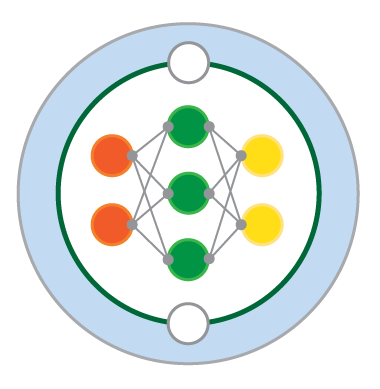
In 1996, Lorenz proposed a two-time scale dynamical system, referred to as the Lorenz-96 model (L96), whose behavior mimics the non-linear dynamics of the extratropical atmosphere with simplified representation of multiscale interactions and nonlinear advection [Lorenz, 1995]. The L96 model consists of two sets of equations coupling two sets of variables (\(X_k\) and \(Y_{j,k}\)), which evolve over two (slow and fast) timescales and are arranged around a latitude circle as shown in Fig. 1. The equations comprising L96 are:
where \(X_k\), \(k=1,\ldots,K\), denotes \(K\) slow (or low-frequency) variables, and \(Y_{j,k}\) , \(j=1,\ldots,J\) denotes \(J*K\) fast (or high-frequency) variables. The slow equations are coupled to the fast equations via a coupling term, \(\sum_{j=0}^{J-1} Y_{j,k}\), which sums over the \(J\) fast variables corresponding to a particular \(k\). On the other hand, each fast equation is forced by a coupling term, \(\frac{hc}{b} X_k\), that depends on the slow variable corresponding to that particular \(k\).
The evolution of this two-time scale system depend on three key parameters: \(b\), \(c\) and \(h\). Here \(b\) determines the magnitude of the nonlinear interactions among the fast variables, \(c\) controls how rapidly the fast variables fluctuate compared to the slow variables and, \(h\) governs the strength of the coupling between the slow and fast variables. Moreover, the slow time-scale equation is forced by the parameter \(F\), whose value determines the chaotic behaviour of the system. E.g. [Wilks, 2005].
The chaotic dynamical system L96 is very useful for testing different numerical methods in atmospheric modeling thanks to its transparency, low computational cost and simplicity compared to Global Climate Models (GCM). The interaction between variables of different scales makes the L96 model of particular interest when evaluating new parameterization methodologies. As such, it was used in assessing different techniques that were later incorporated into GCMs ([Crommelin and Vanden-Eijnden, 2008], [Dorrestijn et al., 2013]).
The L96 model has been extensively used as a test bed in various studies including data assimilation approaches ([Law et al., 2016], [Hatfield et al., 2017]), stochastic parameterization schemes ([Kwasniok, 2012], [Arnold et al., 2013], [Chorin and Lu, 2015]) and Machine Learning-based parameterization methodologies ([Schneider et al., 2017], [Dueben and Bauer, 2018] , [Gagne et al., 2020]).

Fig. 1 Visualisation of a two-scale Lorenz ‘96 system with J = 8 and K = 6. Global-scale variables (\(X_k\)) are updated based on neighbouring variables and on the local-scale variables (\(Y_{j,k}\)) associated with the corresponding global-scale variable. Local-scale variabless are updated based on neighbouring variables and the associated global-scale variable. The neighbourhood topology of both local and global-scale variables is circular. Image from Exploiting the chaotic behaviour of atmospheric models with reconfigurable architectures - Scientific Figure on ResearchGate..#
Code to numerically integrate the two time-scale L96 model#
import matplotlib.pyplot as plt
import numpy as np

from utils import display_source
In the L96_model module we provide the function L96_2t_xdot_ydot (shown next) that returns the tendencies (sum of the RHS) for the X and Y equations, as well as the tendency corresponding to the coupling in the X equation, \(-hc/b \sum_{j=0}^{J-1} Y_{j,k}\).
from L96_model import L96_2t_xdot_ydot

display_source(L96_2t_xdot_ydot)
@njit
def L96_2t_xdot_ydot(X, Y, F, h, b, c):
    """
    Calculate the time rate of change for the X and Y variables for the Lorenz '96, two time-scale
    model, equations 2 and 3:
        d/dt X[k] =     -X[k-1] ( X[k-2] - X[k+1] )   - X[k] + F - h.c/b sum_j Y[j,k]
        d/dt Y[j] = -b c Y[j+1] ( Y[j+2] - Y[j-1] ) - c Y[j]     + h.c/b X[k]

    Args:
        X : Values of X variables at the current time step
        Y : Values of Y variables at the current time step
        F : Forcing term
        h : coupling coefficient
        b : ratio of amplitudes
        c : time-scale ratio
    Returns:
        dXdt, dYdt, C : Arrays of X and Y time tendencies, and the coupling term -hc/b*sum(Y,j)
    """

    JK, K = len(Y), len(X)
    J = JK // K
    assert JK == J * K, "X and Y have incompatible shapes"
    Xdot = np.zeros(K)
    hcb = (h * c) / b

    Ysummed = Y.reshape((K, J)).sum(axis=-1)

    Xdot = np.roll(X, 1) * (np.roll(X, -1) - np.roll(X, 2)) - X + F - hcb * Ysummed
    Ydot = (
        -c * b * np.roll(Y, -1) * (np.roll(Y, -2) - np.roll(Y, 1))
        - c * Y
        + hcb * np.repeat(X, J)
    )

    return Xdot, Ydot, -hcb * Ysummed
These tendencies describe the continuous evolution of the L96 model at a particular time. However, to obtain a discrete solution we must integrate numerically in time. In the L96_model module, we provide the function integrate_L96_2t (shown next) that uses fourth-order Runge-Kutta integration. Starting from the initial conditions X0,Y0, the function returns the trajectories of X,Y sampled at an interval si. There is a related function, integrate_L96_2t_with_coupling, that in addition to the trajectories, also returns the coupling term, \(-hc/b \sum_{j=0}^{J-1} Y_{j,k}\) at each point in the trajectory.
from L96_model import integrate_L96_2t

display_source(integrate_L96_2t)
def integrate_L96_2t(X0, Y0, si, nt, F, h, b, c, t0=0, dt=0.001):
    """
    Integrates forward-in-time the two time-scale Lorenz 1996 model, using the RK4 integration method.
    Returns the full history with nt+1 values starting with initial conditions, X[:,0]=X0 and Y[:,0]=Y0,
    and ending with the final state, X[:,nt+1] and Y[:,nt+1] at time t0+nt*si.

    Note the model is intergrated

    Args:
        X0 : Values of X variables at the current time
        Y0 : Values of Y variables at the current time
        si : Sampling time interval
        nt : Number of sample segments (results in nt+1 samples incl. initial state)
        F  : Forcing term
        h  : coupling coefficient
        b  : ratio of amplitudes
        c  : time-scale ratio
        t0 : Initial time (defaults to 0)
        dt : The actual time step. If dt<si, then si is used. Otherwise si/dt must be a whole number. Default 0.001.

    Returns:
        X[:,:], Y[:,:], time[:] : the full history X[n,k] and Y[n,k] at times t[n]

    Example usage:
        X,Y,t = integrate_L96_2t(5+5*np.random.rand(8), np.random.rand(8*4), 0.01, 500, 18, 1, 10, 10)
        plt.plot( t, X);
    """

    xhist, yhist, time, _ = integrate_L96_2t_with_coupling(
        X0, Y0, si, nt, F, h, b, c, t0=t0, dt=dt
    )

    return xhist, yhist, time
An example of how to use integrate_L96_2t is shown below. Here we choose \(K=36\) and \(J=10\) (i.e. 36 values of \(X\) and 10 values of \(Y\) per value of \(X\)). Also, in accordance with previous studies, we set \(h=1\), \(c=10\), and \(b=10\). The initial condition for \(X\) is setup as \(X(s)=s(s-1)(s+1)\), for \(s=-1\ldots 1\), and the \(Y\) is initialized with zeros. The value of \(F\) is set to \(10\), which is sufficient to obtain chaotic behavior.
Note: if you increase \(F\), you may need to reduce \(dt\) for numerical stability.
K = 36  # Number of globa-scale variables X
J = 10  # Number of local-scale Y variables per single global-scale X variable
nt = 1000  # Number of time steps
si = 0.005  # Sampling time interval
dt = 0.005  # Time step
F = 10.0  # Focring
h = 1.0  # Coupling coefficient
b = 10.0  # ratio of amplitudes
c = 10.0  # time-scale ratio
def s(k, K):
    """A non-dimension coordinate from -1..+1 corresponding to k=0..K"""
    return 2 * (0.5 + k) / K - 1
k = np.arange(K)  # For coordinate in plots
j = np.arange(J * K)  # For coordinate in plots

# Initial conditions
X_init = s(k, K) * (s(k, K) - 1) * (s(k, K) + 1)
Y_init = 0 * s(j, J * K) * (s(j, J * K) - 1) * (s(j, J * K) + 1)

# "Run" model
X, Y, t = integrate_L96_2t(X_init, Y_init, si, nt, F, h, b, c, dt=dt)
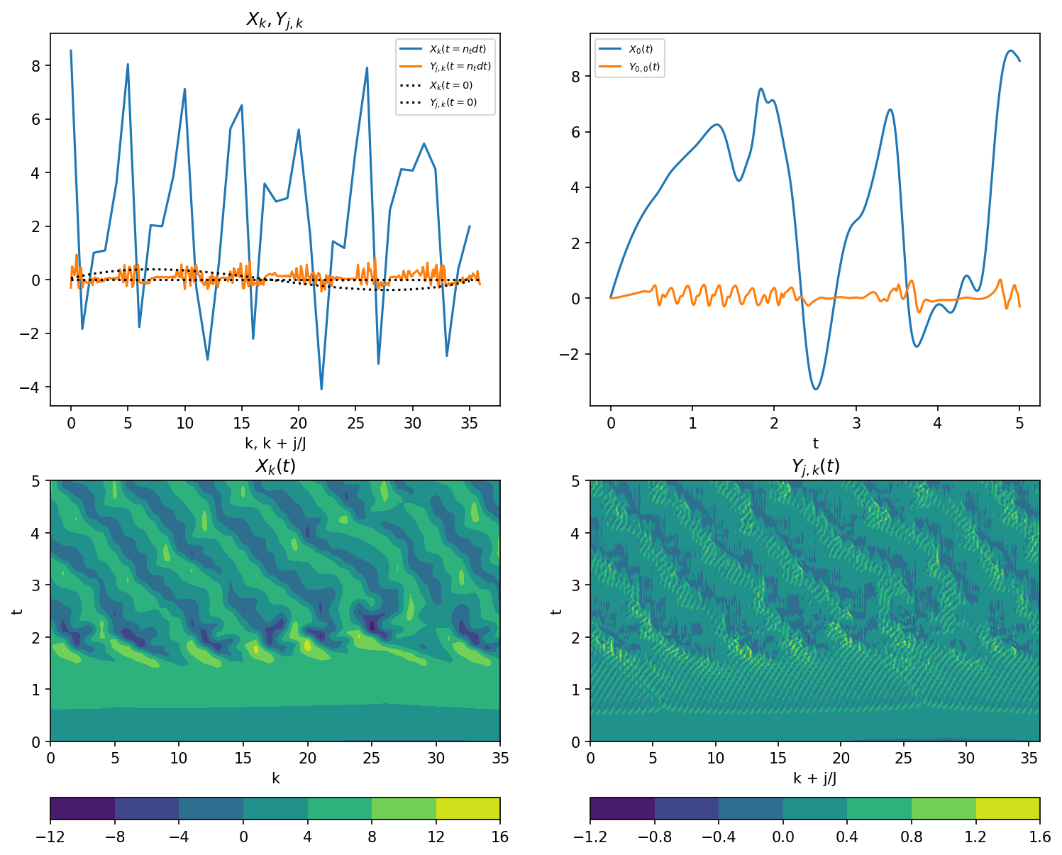
After running the model, we plot the results.
plt.figure(figsize=(12, 10), dpi=150)
plt.subplot(221)

# Snapshot of X[k]
plt.plot(k, X[-1], label="$X_k(t=n_t dt)$")
plt.plot(j / J, Y[-1], label="$Y_{j,k}(t=n_t dt)$")
plt.plot(k, X_init, "k:", label="$X_k(t=0)$")
plt.plot(j / J, Y_init, "k:", label="$Y_{j,k}(t=0)$")
plt.legend(fontsize=7)
plt.xlabel("k, k + j/J")
plt.title("$X_k, Y_{j,k}$")
plt.subplot(222)

# Sample time-series X[0](t), Y[0](t)
plt.plot(t, X[:, 0], label="$X_0(t)$")
plt.plot(t, Y[:, 0], label="$Y_{0,0}(t)$")
plt.legend(fontsize=7)
plt.xlabel("t")
plt.subplot(223)

# Full model history of X
plt.contourf(k, t, X)
plt.colorbar(orientation="horizontal")
plt.xlabel("k")
plt.ylabel("t")
plt.title("$X_k(t)$")
plt.subplot(224)

# Full model history of Y
plt.contourf(j / J, t, Y)
plt.colorbar(orientation="horizontal")
plt.xlabel("k + j/J")
plt.ylabel("t")
plt.title("$Y_{j,k}(t)$");
A class for numerical integration of the two time-scale L96#
For convenience, we also provide a class named L96 in L96_model.py which helps to reduce the amount of code when using the L96_2t_xdot_ydot function.
from L96_model import L96

help(L96)
Help on class L96 in module L96_model:

class L96(builtins.object)
 |  L96(K, J, F=18, h=1, b=10, c=10, t=0, dt=0.001)
 |
 |  Class for two time-scale Lorenz 1996 model
 |
 |  Methods defined here:
 |
 |  __init__(self, K, J, F=18, h=1, b=10, c=10, t=0, dt=0.001)
 |      Construct a two time-scale model with parameters:
 |      K  : Number of X values
 |      J  : Number of Y values per X value
 |      F  : Forcing term (default 18.)
 |      h  : coupling coefficient (default 1.)
 |      b  : ratio of amplitudes (default 10.)
 |      c  : time-scale ratio (default 10.)
 |      t  : Initial time (default 0.)
 |      dt : Time step (default 0.001)
 |
 |  __repr__(self)
 |      Return repr(self).
 |
 |  __str__(self)
 |      Return str(self).
 |
 |  copy(self)
 |
 |  print(self)
 |
 |  randomize_IC(self)
 |      Randomize the initial conditions (or current state)
 |
 |  run(self, si, T, store=False, return_coupling=False)
 |      Run model for a total time of T, sampling at intervals of si.
 |      If store=Ture, then stores the final state as the initial conditions for the next segment.
 |      If return_coupling=True, returns C in addition to X,Y,t.
 |      Returns sampled history: X[:,:],Y[:,:],t[:],C[:,:].
 |
 |  set_param(self, dt=None, F=None, h=None, b=None, c=None, t=None)
 |      Set a model parameter, e.g. .set_param(si=0.01, dt=0.002)
 |
 |  set_state(self, X, Y, t=None)
 |      Set initial conditions (or current state), e.g. .set_state(X,Y)
 |
 |  ----------------------------------------------------------------------
 |  Data descriptors defined here:
 |
 |  __dict__
 |      dictionary for instance variables (if defined)
 |
 |  __weakref__
 |      list of weak references to the object (if defined)
 |
 |  ----------------------------------------------------------------------
 |  Data and other attributes defined here:
 |
 |  F = 'Forcing'
 |
 |  X = 'Current X state or initial conditions'
 |
 |  Y = 'Current Y state or initial conditions'
 |
 |  b = 'Ratio of timescales'
 |
 |  c = 'Ratio of amplitudes'
 |
 |  dt = 'Time step'
 |
 |  h = 'Coupling coefficient'
For example, to setup the same model as above with \(K=36\), \(J=10\) and \(F=10\), use
# Create an instance of the L96 model, default parameters except those given
M = L96(36, 10, F=10, dt=0.005)
M
L96: K=36 J=10 F=10 h=1 b=10 c=10 dt=0.005
Note that parameters \(F\), \(h\), \(b\), \(c\) have defaults since in many of the applications in later notebooks these will not change. The initial conditions are automatically randomized to \(X = b {\cal N}\), \(Y = {\cal N}\) where \({\cal N}\) is a random number drawn from a Guassian distribution. To set the same initial condition as used above, use
# Set the initial conditions (here X is the same cubic as above, Y=0)
M.set_state(s(M.k, M.K) * (s(M.k, M.K) - 1) * (s(M.k, M.K) + 1), 0 * M.j)
print(M)
L96: K=36 J=10 F=10 h=1 b=10 c=10 dt=0.005
 X=[ 0.05326217  0.14641204  0.22258659  0.28281464  0.328125    0.35954647
  0.37810785  0.38483796  0.3807656   0.36691958  0.3443287   0.31402178
  0.27702761  0.234375    0.18709276  0.13620971  0.08275463  0.02775634
 -0.02775634 -0.08275463 -0.13620971 -0.18709276 -0.234375   -0.27702761
 -0.31402178 -0.3443287  -0.36691958 -0.3807656  -0.38483796 -0.37810785
 -0.35954647 -0.328125   -0.28281464 -0.22258659 -0.14641204 -0.05326217]
 Y=[0 0 0 0 0 0 0 0 0 0 0 0 0 0 0 0 0 0 0 0 0 0 0 0 0 0 0 0 0 0 0 0 0 0 0 0 0
 0 0 0 0 0 0 0 0 0 0 0 0 0 0 0 0 0 0 0 0 0 0 0 0 0 0 0 0 0 0 0 0 0 0 0 0 0
 0 0 0 0 0 0 0 0 0 0 0 0 0 0 0 0 0 0 0 0 0 0 0 0 0 0 0 0 0 0 0 0 0 0 0 0 0
 0 0 0 0 0 0 0 0 0 0 0 0 0 0 0 0 0 0 0 0 0 0 0 0 0 0 0 0 0 0 0 0 0 0 0 0 0
 0 0 0 0 0 0 0 0 0 0 0 0 0 0 0 0 0 0 0 0 0 0 0 0 0 0 0 0 0 0 0 0 0 0 0 0 0
 0 0 0 0 0 0 0 0 0 0 0 0 0 0 0 0 0 0 0 0 0 0 0 0 0 0 0 0 0 0 0 0 0 0 0 0 0
 0 0 0 0 0 0 0 0 0 0 0 0 0 0 0 0 0 0 0 0 0 0 0 0 0 0 0 0 0 0 0 0 0 0 0 0 0
 0 0 0 0 0 0 0 0 0 0 0 0 0 0 0 0 0 0 0 0 0 0 0 0 0 0 0 0 0 0 0 0 0 0 0 0 0
 0 0 0 0 0 0 0 0 0 0 0 0 0 0 0 0 0 0 0 0 0 0 0 0 0 0 0 0 0 0 0 0 0 0 0 0 0
 0 0 0 0 0 0 0 0 0 0 0 0 0 0 0 0 0 0 0 0 0 0 0 0 0 0 0]
 t=0
To sample the same tracjectories as above use the .run() method.
# Run the model for 1000 sample intervals, or for time 1000*0.005 = 5
X2, Y2, t = M.run(0.005, 5)

print("Mean absolute difference =", np.abs(X2 - X).mean() + np.abs(Y2 - Y).mean())
Mean absolute difference = 0.0
Re-running the above cell gives the same answer each time because the same initial conditions are used for each invocation or .run(). To allow sequences of run, using the end state of one as the starting point for the next, add the parameter store=True which updates the initial condition stored in the object (M) with the final state of the run.
# Run the model as above but use the end state as an initial condition for the next run.
# (Re-running this cell will give different answers after the first run)
X2, Y2, t = M.run(0.005, 5, store=True)

print(
    "Mean absolute difference 1st run=", np.abs(X2 - X).mean() + np.abs(Y2 - Y).mean()
)

X2, Y2, t = M.run(0.005, 5, store=True)
print(
    "Mean absolute difference 2nd run=", np.abs(X2 - X).mean() + np.abs(Y2 - Y).mean()
)
Mean absolute difference 1st run= 0.0
Mean absolute difference 2nd run= 4.761055522025149
The entire model creation and execution process demonstrated above can also be implemented in a one-liner version as shown below.
X3, Y3, t = (
    L96(36, 10, F=10, dt=0.005)
    .set_state(s(M.k, M.K) * (s(M.k, M.K) - 1) * (s(M.k, M.K) + 1), 0 * M.j)
    .run(0.005, 5)
)