The Lorenz-96 and its GCM Analog

The Lorenz-96 and its GCM Analog#

The physical equations of motion of the system describing the atmosphere dynamics are known. Also in the real atmosphere there is variability over all scales, from the smallest molecular scales to the largest planetary scales. Thus, it is not feasible to explicitly solve the known physical equations of motion within Global Climate Models (GCMs), as computational resources limit the range of scales that can be resolved. To make the behavior of the GCM better match the real world, we need to effectively parameterize the effects that the unresolved scales have on the resolved (large) scales.

The two time-scale L96 model, described in the the previous notebook, can be considered as a simplified analog for real world atmosphere, where variability resides at only two discrete scales (a simplification of the continuum in the real world). In this analogy, a GCM would be a model that can only solve the equations for the slow time scale, where the effects of the fast time-scale variables would be missing. We introduce the single time-scale version of the L96 model below. To make the single time scale model match the two time scale model, the effects of the fast time scales need to parameterized into the single time scale model.

The two time-scale model: Analog for the real atmosphere#

We will first describe a simulation with the two time-scale model from the The Lorenz-96 Two-Timescale System, which is taken as the control simulation that we hope to replicate with the single time-scale model.

The forcing and resolution parameters, \(F\), \(J\) and \(K\), for the two time-scale model are fixed based on [Wilks, 2005], as \(F=18\) or \(20\), \(K=8\), and \(J=32\). Here, the value chosen for the parameter \(F\) is set large enough to ensure chaotic behavior. We also use the reference values for the \(h\), \(b\) and \(c\) parameters to be, \(h=1\), \(b=10\), and \(c=10\). With this particular choice of parameter values, one model time unit (MTU) is approximately equivalent to five atmospheric days. This estimate is obtained by comparing error-doubling times in the Lorenz-96 model and the real atmosphere [Lorenz, 1995].

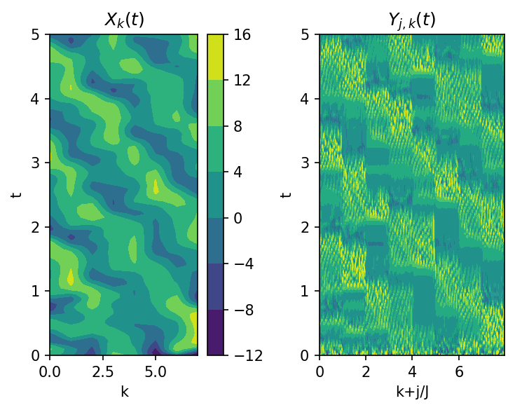
In the following code, we solve the L96 system using an accurate time-stepping scheme (RK4 with sufficiently small \(\Delta t\)), and plot the time evolution for the \(X_k\) and \(Y_{j,k}\) variables.

import numpy as np
import matplotlib.pyplot as plt
from L96_model import L96

np.random.seed(23)
W = L96(8, 32)
T = 5.0
%time X_true,Y_true,t = W.run(0.05, T)

CPU times: user 2.53 s, sys: 32.4 ms, total: 2.57 s
Wall time: 2.57 s

Here is the what the solution looks like:

plt.figure(figsize=(5, 4), dpi=150)

plt.subplot(121)
plt.contourf(W.k, t, X_true)
plt.colorbar()
plt.xlabel("k")
plt.ylabel("t")
plt.title("$X_k(t)$")

plt.subplot(122)
plt.contourf(W.j / W.J, t, Y_true, levels=np.linspace(-1, 1, 10))
plt.xlabel("k+j/J")
plt.ylabel("t")
plt.title("$Y_{j,k}(t)$")

plt.tight_layout()

../_images/8e6fb16b88b45800be7e1ddcb232672d663071c8b0b17df5eae198b2453fb025.png

The single time-scale model: Analog for a general circulation model (GCM)#

The two time-scale model discussed above solves a set of equations for the slow and fast variables, where the equations for the slow variables are:

(2)#\[\begin{align} \frac{d}{dt} X_k &= - X_{k-1} \left( X_{k-2} - X_{k+1} \right) - X_k + F - \underbrace{ \left( \frac{hc}{b} \right) \sum_{j=0}^{J-1} Y_{j,k} }_{=U_k} \ . \end{align}\]

Here the effects of the fast scales on the slow scales are represented by the last term on the RHS, denoted as \(U_k\), \(k=1,\ldots,k\).

In the single time-scale model the explicit equations for the fast scales are not known, and so we do not know what \(Y_{j,k}\) or subsequently \(U_k\) are. So, in the single time-scale model the effects of the fast scales are either missing, \(U_k=0\), or they need to be specified/parameterized purely in terms of the known slow time-scale variables, \(U_k \approx P (X_k)\).

In the following code, we show how the single time scale model can be solved. We use L96_eq1_xdot (code shown below), which returns the tendency (RHS) corresponding to the following equation, where there are no coupling or parameterization terms,

(3)#\[\begin{align} \frac{d}{dt} X_k &= - X_{k-1} \left( X_{k-2} - X_{k+1} \right) - X_k + F. \end{align}\]

from L96_model import L96_eq1_xdot
from utils import display_source

display_source(L96_eq1_xdot)

@njit
def L96_eq1_xdot(X, F, advect=True):
    """
    Calculate the time rate of change for the X variables for the Lorenz '96, equation 1:
        d/dt X[k] = -X[k-2] X[k-1] + X[k-1] X[k+1] - X[k] + F

    Args:
        X : Values of X variables at the current time step
        F : Forcing term
    Returns:
        dXdt : Array of X time tendencies
    """

    K = len(X)
    Xdot = np.zeros(K)

    if advect:
        Xdot = np.roll(X, 1) * (np.roll(X, -1) - np.roll(X, 2)) - X + F
    else:
        Xdot = -X + F
    #     for k in range(K):
    #         Xdot[k] = ( X[(k+1)%K] - X[k-2] ) * X[k-1] - X[k] + F
    return Xdot

Now we define GCM, which solves for the temporal evolution of \(X\)s using a simple Euler integration.

#  We define the GCM which solves for X in time and returns its time series
def GCM(X0, F, dt, nt, param=[0]):
    time, hist, X = dt * np.arange(nt), np.zeros((nt, len(X0))) * np.nan, X0.copy()

    for n in range(nt):
        X = X + dt * (L96_eq1_xdot(X, F) - np.polyval(param, X))
        if np.abs(X).max() > 1e3:
            break
        hist[n], time[n] = X, dt * (n + 1)
    return hist, time

Notice that we have added the possibility of adding a parameterization that may take the form a polynomial function, this will be discussed futher below.

X_init, dt, F_mod = X_true[0], 0.002, W.F
# set the initial condition to be the same
# we also set the dt to be smaller as the Euler scheme is less accurate

# no parameterization
X_gcm_no_param, T_gcm_no_param = GCM(X_init, F_mod, dt, int(T / dt))

plt.figure(figsize=(2.5, 4), dpi=150)

plt.subplot(111)
plt.contourf(W.k, T_gcm_no_param, X_gcm_no_param)
plt.colorbar()
plt.xlabel("k")
plt.ylabel("t")
plt.title("$X_k(t)$")

plt.tight_layout()

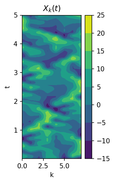
../_images/4ff447a44162aad66fe5cf9a70bed8be64046d13bc8fd8a677b2bd0b61099983.png

Clearly, the evolution the single time scale system does not even qualitatively match the evolution of the two time scale system. For example, the leftward propagation is completely missing.

Adding a parametization to the single time-scale model#

The single time-scale model does not behave the same as the two time-scale model, since the effects of the fast time-scales (or “unresolved scales” or “sub-grid effects” or “sub-grid tendencies”) are missing. To obtain a closer match to the two time-scale model, we need to introduce these missing effects into the single time-scale model. Adding these missing effects is known as parameterization, where the effect of the missing scales are represented purely in terms of the variables that are known in the gcm (\(X\)’s only in the single time-scale model).

The one time-scale equation of the Lorenz-96 model with a parameterization for the effects of the fast time-scale , can be written as:

(4)#\[\begin{align} \frac{d}{dt} X_k &= - X_{k-1} \left( X_{k-2} - X_{k+1} \right) - X_k + F - P\left( X_k \right) \ . \end{align}\]

Here, we consider a particular functional form for modeling the unknown parameterization, using a polynomial approximation. Example of such a parameterization include the fourth-order polynomial form proposed by [Wilks, 2005]:

\[\begin{equation*} P(X_k)=b_0 + b_1 X_k + b_2 X_k^2 + b_3 X_k^3 + b_4 X_k^4 + e_k. \end{equation*}\]

Alternatively, we also consider a first-order polynomial as suggested by [Arnold et al., 2013]:

\[\begin{equation*} P(X_k)=b_0 + b_1 X_k + e_k. \end{equation*}\]

In both these forms \(e_k\) is a stochastic component, which will not be discussed further till the next notebook.

All parameterizations have some unknown parameters, which need to be determined in some way. These parameters may be guessed based on some intuition about the physics, or determined from data collected in the real system (two time-scale model here), or optimized to make the evolution of the reduced (single time-scale) model match the evolution of the real world or full (two time-scale model) model. In this notebook we will use the second approach, and the last approach will be discussed in Tuning GCM Parameterizations.

In summary: with the “real atmosphere” or two time-scale system in hand, we can “observe” the effect of the sub-grid forcing on the large scale (\(U_k\)) and test the skill of the polynomial function, \(P(X_k)\), models/parameterizations.

%time X, Y, t = W.run(0.05, 200.) # We first run the 2 time-scale model again for longer time, to generate more data.

CPU times: user 7.81 s, sys: 4.12 ms, total: 7.81 s
Wall time: 7.8 s

X_copy = X
# Generate U_k samples from 2 time-scale model
# using the longer time series, we now generate samples of U_k that are used to
# estimate the unknown parameters.
U_sample = (W.h * W.c / W.b) * Y.reshape((Y.shape[0], W.K, W.J)).sum(axis=-1)

# Fit polynomial of order 1.
p1 = np.polyfit(
    X_copy.flatten(), U_sample.flatten(), 1
)  # Fit a linear curve through the data.
print("Linear Poly coeffs:", p1)

# We use the parameters from from Wilks, 2005
p4 = [
    0.000707,
    -0.0130,
    -0.0190,
    1.59,
    0.275,
]
# We could have just as easily have fit the parameters using the data as well.

Linear Poly coeffs: [0.85439536 0.75218026]

We now compare the results obtained with a linear polynomial approximation, Wilks [2005] polynomial parameterization and the “truth” values of the coupling terms.

plt.figure(dpi=150)
# 2D histogram of X vs U
plt.hist2d(X_copy.flatten(), U_sample.flatten(), bins=50, density=True)
plt.xlabel("$X_k$")
plt.ylabel(r"$U_k = \frac{hc}{b}\sum_j Y_{j,k}$")
plt.colorbar(label="PDF")

# Fits from polynomials
x = np.linspace(-12, 18, 100)
plt.plot(x, np.polyval(p4, x), label="$P_4(X_k)$ - Wilks, 2005")
plt.plot(x, np.polyval(p1, x), "--", label="$P_1(X_k)$")


plt.legend(fontsize=7);

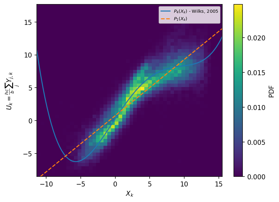
../_images/c20856426db6571b7afff12caee3a80fd0e2ee35f918c1995f9cfc0162d4584a.png

The figure above shows that the the relationship between the slow variables (\(X_k\)) and the observed coupling term (\(U_k\)) is non-linear. The higher order polynomlial, since it is more flexible, does a better job at capturing the overall pattern, relative to the linear fit.

We had already setup the code in GCM to accept polynomial parameterizations, which can be turned on by passing the parameters. We will use this in the next section to test the effect that the parameterization has on the single time-scale model.

Testing the effect of parameterizations in the “GCM” model#

Now that we have a couple of different candidate parameterizations that can roughly predict the relationship between the slow variables and sub-grid forcing, we test their impact in a GCM simulation where the parameterization is required. We compare four simulations:

“Real world”: corresponding to the “truth” model goverened by the full two time-scale Lorenz-96 system.
GCM without parameterization: corresponding to the one time-scale Lorenz-96 system without any the coupling term. We use a forward-Euler scheme to integrate the model forward.
GCM with our parameterization: corresponding to the one time-scale Lorenz-96 system with the linear polynomial approximation of the coupling terms as obtained above.
GCM with [Wilks, 2005] parameterization: corresponding to the one time-scale Lorenz-96 system with a third-order polynomial approximation of the coupling terms.

np.random.seed(13)
T = 5
# Real world
X_true, Y_true, T_true = W.randomize_IC().run(0.05, T)
X_init, dt, F_mod = X_true[0] + 0.0 * np.random.randn(W.K), 0.002, W.F + 0.0
# The reason for adding the zero terms to X and F will become clear below, where the amplitude will be increased.

# no parameterization
X_gcm1, T_gcm1 = GCM(X_init, F_mod, dt, int(T / dt))
# Linear parameterization
X_gcm2, T_gcm2 = GCM(X_init, F_mod, dt, int(T / dt), param=p1)
# Wilks parameterization - 4th order polynomial.
X_gcm3, T_gcm3 = GCM(X_init, F_mod, dt, int(T / dt), param=p4)

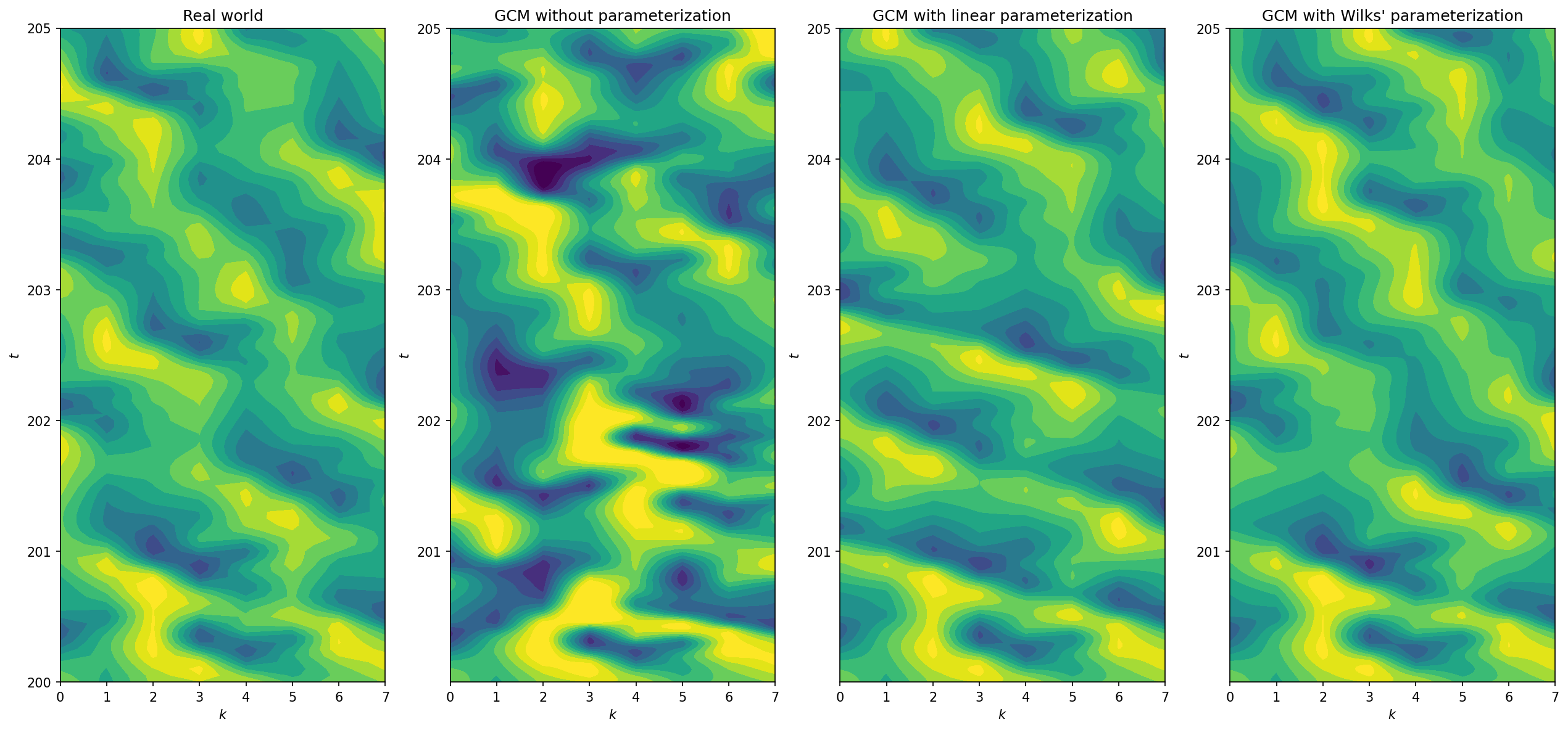
Now we look at Hovmoeller plots of the different solutions.

plt.figure(dpi=150, figsize=(17, 8))
lims = {"vmin": -12, "vmax": 12, "levels": np.linspace(-12, 12, 12), "extend": "both"}
plt.subplot(141)
plt.contourf(W.k, T_true + t[-1], X_true, **lims)
plt.xlabel("$k$")
plt.ylabel("$t$")
plt.title("Real world")
plt.subplot(142)
plt.contourf(W.k, T_gcm1 + t[-1], X_gcm1, **lims)
plt.xlabel("$k$")
plt.ylabel("$t$")
plt.title("GCM without parameterization")
plt.subplot(143)
plt.contourf(W.k, T_gcm3 + t[-1], X_gcm2, **lims)
plt.xlabel("$k$")
plt.ylabel("$t$")
plt.title("GCM with linear parameterization")
plt.subplot(144)
plt.contourf(W.k, T_gcm2 + t[-1], X_gcm3, **lims)
plt.xlabel("$k$")
plt.ylabel("$t$")
plt.title("GCM with Wilks' parameterization")

plt.tight_layout()

../_images/f72abcd2b030ce1152a4aa1e0cf3e7e2cc412457a41511880743bc9a595b4411.png

The next plot shows the temporal evolution of the variable \(X_3\) obtained with the four models listed above.

k = 3
plt.figure(dpi=150)
plt.plot(T_true + t[-1], X_true[:, k], "--", label="Real world")
plt.plot(T_gcm1 + t[-1], X_gcm1[:, k], ":", label="GCM without parameterization")
plt.plot(T_gcm1 + t[-1], X_gcm2[:, k], label="GCM with our parameterization")
plt.plot(T_gcm1 + t[-1], X_gcm3[:, k], label="GCM with Wilks parameterization")
plt.xlabel("$t$")
plt.ylabel("$X_3(t)$")
plt.legend(fontsize=7, loc=1)
plt.ylim(-10, 25);

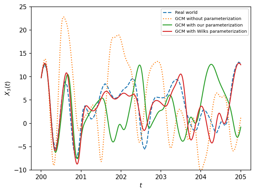
../_images/d8e6ca354b9326e866c7705704354e0856e80cc51ccfc27d777a382cc016429c.png

As seen above, all the simulation diverge at long times,and the unparameterized simulation diverges very rapidly. On the other hand, the parameterized GCMs track the “real world” solution better. The Wilks parameterization does better than the linear fit.

Summary#

In this chapter:

We argued that the single time-scale L96 model is a reduced representation of the two time-scale L96 model, which can be considered analogous to the way GCMs are a reduced repseration of the real world.
We showed that missing effects need to be parameterized, if the reduced representation is required behave like the full model/real world.
We used the two time-scale L96 model to generate a “truth” dataset for the effects of unresolved scales.
We built a “GCM” with a polynomial parameterization of coupling to unresolved processes (\(\left( \frac{hc}{b} \right) \sum_{j=0}^{J-1} Y_{j,k}\))
Finally we compared the solution from the two time-scale, single time-scale and parameterized single time-scale models, showing that the paramaterized version evolves more similarly to the two time-scale model.

In the next chapter we will further explore some key properties of parameterizations, and also discuss the other sources of error that can lead to a difference between the reduced and full models (or GCMs and real world).