ResNet and Recurrent Neural Networks

%matplotlib inline
from matplotlib.animation import FuncAnimation
from IPython.display import HTML
import numpy as np
import matplotlib.pyplot as plt
import math
import pandas as pd

import torch
from torch.autograd import Variable
import torch.nn.functional as F
import torch.utils.data as Data
import torchvision
from torch import nn, optim

# from torch_lr_finder import LRFinder
import torch.nn.functional as F
from torch import nn
from L96_model import L96, L96_eq1_xdot, integrate_L96_2t, EulerFwd, RK2, RK4

Lorenz (1996) describes a “two time-scale” model in two equations (2 and 3) which are:

(51)\[\begin{align} \frac{d}{dt} X_k &= - X_{k-1} \left( X_{k-2} - X_{k+1} \right) - X_k + F - \left( \frac{hc}{b} \right) \sum_{j=0}^{J-1} Y_{j,k} \\ \frac{d}{dt} Y_{j,k} &= - cbY_{j+1,k} \left( Y_{j+2,k} - Y_{j-1,k} \right) - c Y_{j,k} + \frac{hc}{b} X_k \end{align}\]

Fig. 10 Visualisation of a two-scale Lorenz ‘96 system with J = 8 and K = 6. Global-scale variables (\(X_k\)) are updated based on neighbouring variables and on the local-scale variables (\(Y_{j,k}\)) associated with the corresponding global-scale variable. Local-scale variabless are updated based on neighbouring variables and the associated global-scale variable. The neighbourhood topology of both local and global-scale variables is circular. Image from Exploiting the chaotic behaviour of atmospheric models with reconfigurable architectures - Scientific Figure on ResearchGate..

Generating data from L96:

time_steps = 20000
Forcing, dt, T = 18, 0.01, 0.01 * time_steps

# Create a "real world" with K=8 and J=32
W = L96(8, 32, F=Forcing)

# Get training data for the neural network.
# - Run the true state and output subgrid tendencies (the effect of Y on X is xytrue):
X_true, y, t, xy_true = W.run(dt, T, return_coupling=True)

val_size = 4000  # number of time steps for validation
# train:
X_true_train = X_true[
    :-val_size, :
]  # Flatten because we first use single input as a sample
subgrid_tend_train = xy_true[:-val_size, :]

# test:
X_true_test = X_true[-val_size:, :]
subgrid_tend_test = xy_true[-val_size:, :]

# Create non local training data
# Define a data loader (8 inputs, 8 outputs)

# Define our X,Y pairs (state, subgrid tendency) for the linear regression local network.local_torch_dataset = Data.TensorDataset(
torch_dataset = Data.TensorDataset(
    torch.from_numpy(X_true_train).double(),
    torch.from_numpy(subgrid_tend_train).double(),
)

BATCH_SIZE = 1024  # Number of sample in each batch

loader = Data.DataLoader(dataset=torch_dataset, batch_size=BATCH_SIZE, shuffle=True)

# Define a test dataloader (8 inputs, 8 outputs)

torch_dataset_test = Data.TensorDataset(
    torch.from_numpy(X_true_test).double(), torch.from_numpy(subgrid_tend_test).double()
)

loader_test = Data.DataLoader(
    dataset=torch_dataset_test, batch_size=BATCH_SIZE, shuffle=True
)

(52)\[\begin{align} \frac{d}{dt} X_k &= - X_{k-1} \left( X_{k-2} - X_{k+1} \right) - X_k + F - \left( \frac{hc}{b} \right) \sum_{j=0}^{J-1} Y_{j,k} \\ \frac{d}{dt} Y_{j,k} &= - cbY_{j+1,k} \left( Y_{j+2,k} - Y_{j-1,k} \right) - c Y_{j,k} + \frac{hc}{b} X_k \end{align}\]

Goal: Use \(X_k\) to predict subgrid terms, \(- \left( \frac{hc}{b} \right) \sum_{j=0}^{J-1} Y_{j,k}\)

Janni’s fully connected, 3-layer Artificial Neural Network (ANN)

K=8 and J=32

class Net_ANN(nn.Module):
    def __init__(self):
        super(Net_ANN, self).__init__()
        self.linear1 = nn.Linear(8, 16)  # 8 inputs, 16 neurons for first hidden layer
        self.linear2 = nn.Linear(16, 16)  # 16 neurons for second hidden layer
        self.linear3 = nn.Linear(16, 8)  # 8 outputs

    #         self.lin_drop = nn.Dropout(0.1) #regularization method to prevent overfitting.

    def forward(self, x):
        x = F.relu(self.linear1(x))
        x = F.relu(self.linear2(x))
        x = self.linear3(x)
        return x

def train_model(net, criterion, trainloader, optimizer):
    net.train()
    test_loss = 0
    for step, (batch_x, batch_y) in enumerate(trainloader):  # for each training step
        b_x = Variable(batch_x)  # Inputs
        b_y = Variable(batch_y)  # outputs
        if (
            len(b_x.shape) == 1
        ):  # If is needed to add a dummy dimension if our inputs are 1D (where each number is a different sample)
            prediction = torch.squeeze(
                net(torch.unsqueeze(b_x, 1))
            )  # input x and predict based on x
        else:
            prediction = net(b_x)
        loss = criterion(prediction, b_y)  # Calculating loss
        optimizer.zero_grad()  # clear gradients for next train
        loss.backward()  # backpropagation, compute gradients
        optimizer.step()  # apply gradients to update weights

def test_model(net, criterion, trainloader, optimizer, text="validation"):
    net.eval()  # Evaluation mode (important when having dropout layers)
    test_loss = 0
    with torch.no_grad():
        for step, (batch_x, batch_y) in enumerate(
            trainloader
        ):  # for each training step
            b_x = Variable(batch_x)  # Inputs
            b_y = Variable(batch_y)  # outputs
            if (
                len(b_x.shape) == 1
            ):  # If is needed to add a dummy dimension if our inputs are 1D (where each number is a different sample)
                prediction = torch.squeeze(
                    net(torch.unsqueeze(b_x, 1))
                )  # input x and predict based on x
            else:
                prediction = net(b_x)
            loss = criterion(prediction, b_y)  # Calculating loss
            test_loss = test_loss + loss.data.numpy()  # Keep track of the loss
        test_loss /= len(trainloader)  # dividing by the number of batches
    #         print(len(trainloader))
    # disabling prints to only show graphs
    # print(text + ' loss:',test_loss)
    return test_loss

criterion = torch.nn.MSELoss()  # MSE loss function

nn_3l = Net_ANN().double()
# optimizer = optim.Adam(nn_3l.parameters(), lr=1e-7)
# lr_finder = LRFinder(nn_3l, optimizer, criterion)
# lr_finder.range_test(loader, end_lr=100, num_iter=200)
# lr_finder.plot() # to inspect the loss-learning rate graph
# lr_finder.reset() # to reset the model and optimizer to their initial state

n_epochs = 20  # Number of epocs
optimizer = optim.Adam(nn_3l.parameters(), lr=0.01)
validation_loss = list()
train_loss = list()
# time0 = time()
for epoch in range(1, n_epochs + 1):
    train_model(nn_3l, criterion, loader, optimizer)
    train_loss.append(test_model(nn_3l, criterion, loader, optimizer, "train"))
    validation_loss.append(test_model(nn_3l, criterion, loader_test, optimizer))
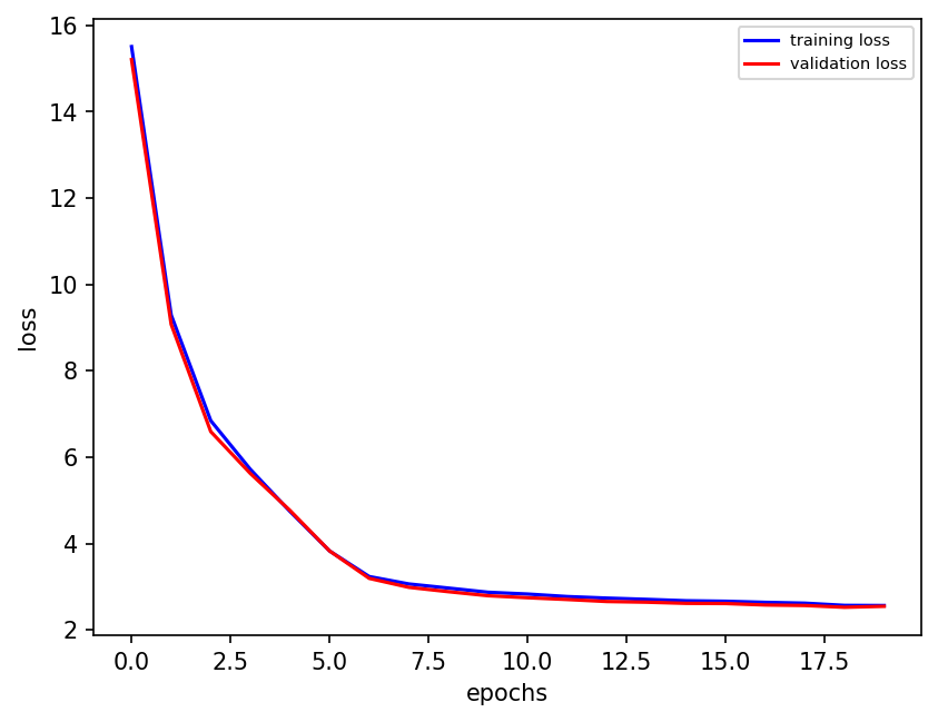
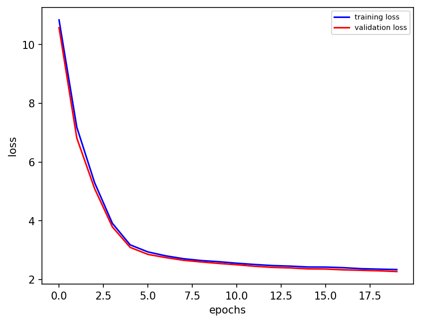
plt.figure(dpi=150)
plt.plot(train_loss, "b", label="training loss")
plt.plot(validation_loss, "r", label="validation loss")
plt.ylabel("loss")
plt.xlabel("epochs")
plt.legend(fontsize=7)

final_losses = np.zeros(4)
final_losses[0] = validation_loss[-1]

preds22 = nn_3l(torch.from_numpy(X_true_test[:, :]).double())
plt.figure(dpi=150)
plt.plot(preds22.detach().numpy()[0:1000, 1], label="NN Predicted values")
plt.plot(subgrid_tend_test[:1000, 1], label="True values")

plt.legend(fontsize=7);

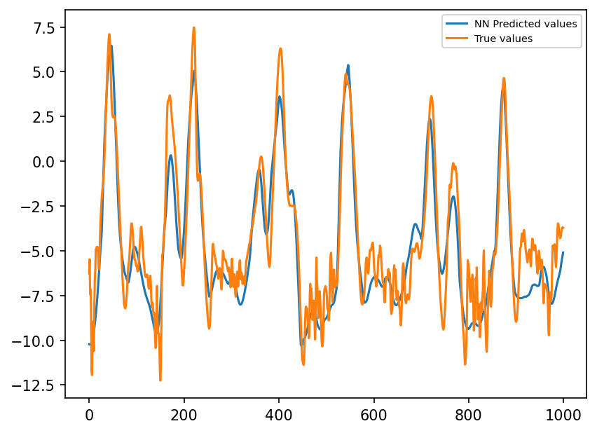
3-layer ANN is (too) good!

ResNet

ResNet is based on residual blocks, depicted below
Residual blocks are based on skip connections
Skip connections add output from one layer to that of a deeper layer

ResNet is famously applied to image recognition using NN that are very deep

He, Kaiming, et al. “Deep Residual Learning for Image Recognition.” ArXiv.org, 2015, arxiv.org/abs/1512.03385. Accessed 5 Oct. 2021.

Pretrained image recognition ResNet models are available with tens or >100 layers
This is not our use case for Lorenz ‘96

However, adaptation for dynamic systems do exist, e.g. https://towardsdatascience.com/neural-odes-breakdown-of-another-deep-learning-breakthrough-3e78c7213795\

Here, we’ll look at skip connections and residual blocks, rather than ResNet
First, need to ‘break’ Janni’s model by adding too many layers

class Net_deepNN(nn.Module):
    def __init__(self):
        super(Net_deepNN, self).__init__()
        self.linear1 = nn.Linear(8, 16)  # 8 inputs, 16 neurons for first hidden layer
        self.linear2 = nn.Linear(16, 16)  # 16 neurons for second hidden layer
        self.linear3 = nn.Linear(16, 16)
        self.linear4 = nn.Linear(16, 16)
        self.linear5 = nn.Linear(16, 16)
        self.linear6 = nn.Linear(16, 8)  # 8 outputs

    #         self.lin_drop = nn.Dropout(0.1) #regularization method to prevent overfitting.

    def forward(self, x):
        x = F.relu(self.linear1(x))
        x = F.relu(self.linear2(x))
        x = F.relu(self.linear3(x))
        x = F.relu(self.linear4(x))
        x = F.relu(self.linear5(x))
        x = self.linear6(x)
        return x

nn_deep = Net_deepNN().double()
# optimizer = optim.Adam(nn_deep.parameters(), lr=1e-7)
# lr_finder = LRFinder(nn_deep, optimizer, criterion)
# lr_finder.range_test(loader, end_lr=100, num_iter=200)
# lr_finder.plot() # to inspect the loss-learning rate graph
# lr_finder.reset() # to reset the model and optimizer to their initial state

n_epochs = 40  # Number of epocs
optimizer = optim.Adam(nn_deep.parameters(), lr=0.01)
validation_loss = list()
train_loss = list()
# time0 = time()
for epoch in range(1, n_epochs + 1):
    train_model(nn_deep, criterion, loader, optimizer)
    train_loss.append(test_model(nn_deep, criterion, loader, optimizer, "train"))
    validation_loss.append(test_model(nn_deep, criterion, loader_test, optimizer))
plt.figure(dpi=150)
plt.plot(train_loss, "b", label="training loss")
plt.plot(validation_loss, "r", label="validation loss")
plt.ylabel("loss")
plt.xlabel("epochs")
plt.legend(fontsize=7)

final_losses[1] = validation_loss[-1]

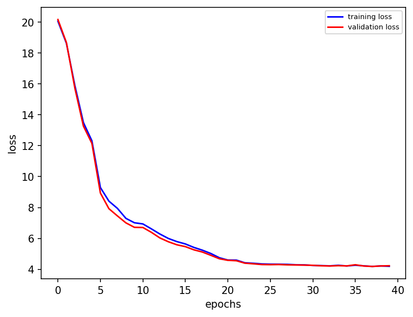
Worse loss with twice the training epochs

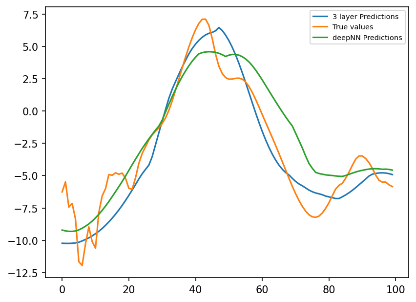
preds_deep = nn_deep(torch.from_numpy(X_true_test[:, :]).double())
plt.figure(dpi=150)
plt.plot(preds22.detach().numpy()[0:100, 1], label="3 layer Predictions")
plt.plot(subgrid_tend_test[:100, 1], label="True values")
plt.plot(preds_deep.detach().numpy()[0:100, 1], label="deepNN Predictions")
plt.legend(fontsize=7);

class Net_deepNN_withSkips(nn.Module):
    def __init__(self):
        super(Net_deepNN_withSkips, self).__init__()
        self.linear1 = nn.Linear(8, 16)  # 8 inputs, 16 neurons for first hidden layer
        self.linear2 = nn.Linear(16, 16)  # 16 neurons for second hidden layer
        self.linear3 = nn.Linear(16, 16)
        self.linear4 = nn.Linear(16, 16)
        self.linear5 = nn.Linear(16, 16)
        self.linear6 = nn.Linear(16, 8)  # 8 outputs

    #         self.lin_drop = nn.Dropout(0.1) #regularization method to prevent overfitting.

    def forward(self, x):
        x1 = F.relu(self.linear1(x))
        x2 = F.relu(self.linear2(x1))
        x3 = F.relu(self.linear3(x2)) + x1
        x4 = F.relu(self.linear4(x3))
        x5 = F.relu(self.linear5(x4)) + x3
        x6 = self.linear6(x5)
        return x6

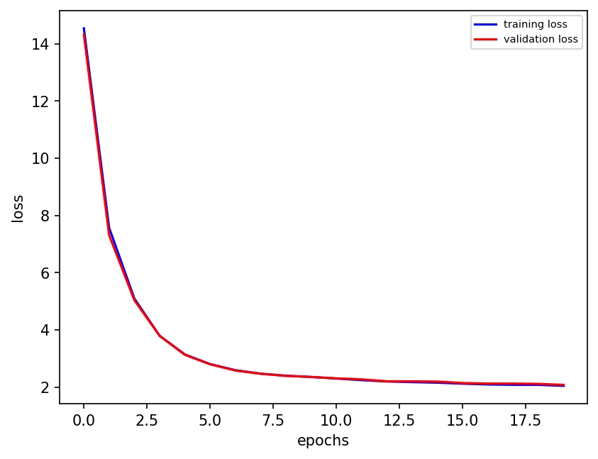
nn_deep_skips = Net_deepNN_withSkips().double()

n_epochs = 20  # Number of epocs
optimizer = optim.Adam(nn_deep_skips.parameters(), lr=0.01)
validation_loss = list()
train_loss = list()
# time0 = time()
for epoch in range(1, n_epochs + 1):
    train_model(nn_deep_skips, criterion, loader, optimizer)
    train_loss.append(test_model(nn_deep_skips, criterion, loader, optimizer, "train"))
    validation_loss.append(test_model(nn_deep_skips, criterion, loader_test, optimizer))
plt.figure(dpi=150)
plt.plot(train_loss, "b", label="training loss")
plt.plot(validation_loss, "r", label="validation loss")
plt.ylabel("loss")
plt.xlabel("epochs")
plt.legend(fontsize=7)

# final_losses=np.append(final_losses,validation_loss[-1])
final_losses[2] = validation_loss[-1]

preds_deep_skips = nn_deep_skips(torch.from_numpy(X_true_test[:, :]).double())
plt.figure(dpi=150)
plt.plot(preds22.detach().numpy()[0:100, 1], label="3 layer Predictions")
plt.plot(subgrid_tend_test[:100, 1], label="True values")
plt.plot(preds_deep.detach().numpy()[0:100, 1], label="deepNN Predictions")
plt.plot(
    preds_deep_skips.detach().numpy()[0:100, 1], label="deepNN w/ skips Predictions"
)
plt.legend(fontsize=7);

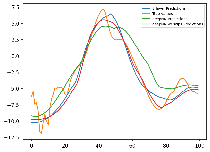
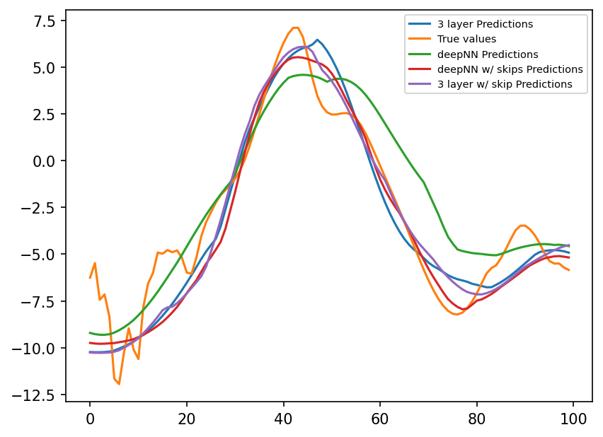
Adding skips led to two improvements

• Improved loss, lower than that of deep network without skips and the original 3-layer NN

• Faster training

class Net_3L_withSkip(nn.Module):
    def __init__(self):
        super(Net_3L_withSkip, self).__init__()
        self.linear1 = nn.Linear(8, 16)  # 8 inputs, 16 neurons for first hidden layer
        self.linear2 = nn.Linear(16, 16)  # 16 neurons for second hidden layer
        self.linear3 = nn.Linear(16, 8)  # 8 outputs

    #         self.lin_drop = nn.Dropout(0.1) #regularization method to prevent overfitting.

    def forward(self, x):
        x = F.relu(self.linear1(x))
        x = F.relu(self.linear2(x)) + x
        x = self.linear3(x)
        return x

nn_3l_skip = Net_3L_withSkip().double()
# optimizer = optim.Adam(nn_3l_res.parameters(), lr=1e-7)
# lr_finder = LRFinder(nn_3l_res, optimizer, criterion)
# lr_finder.range_test(loader, end_lr=100, num_iter=200)
# lr_finder.plot() # to inspect the loss-learning rate graph
# lr_finder.reset() # to reset the model and optimizer to their initial state

n_epochs = 20  # Number of epocs
optimizer = optim.Adam(nn_3l_skip.parameters(), lr=0.01)
validation_loss = list()
train_loss = list()
# time0 = time()
for epoch in range(1, n_epochs + 1):
    train_model(nn_3l_skip, criterion, loader, optimizer)
    train_loss.append(test_model(nn_3l_skip, criterion, loader, optimizer, "train"))
    validation_loss.append(test_model(nn_3l_skip, criterion, loader_test, optimizer))
plt.figure(dpi=150)
plt.plot(train_loss, "b", label="training loss")
plt.plot(validation_loss, "r", label="validation loss")
plt.ylabel("loss")
plt.xlabel("epochs")
plt.legend(fontsize=7)

final_losses[3] = validation_loss[-1]

preds_3l_skip = nn_3l_skip(torch.from_numpy(X_true_test[:, :]).double())
plt.figure(dpi=150)
plt.plot(preds22.detach().numpy()[0:100, 1], label="3 layer Predictions")
plt.plot(subgrid_tend_test[:100, 1], label="True values")
plt.plot(preds_deep.detach().numpy()[0:100, 1], label="deepNN Predictions")
plt.plot(
    preds_deep_skips.detach().numpy()[0:100, 1], label="deepNN w/ skips Predictions"
)
plt.plot(preds_3l_skip.detach().numpy()[0:100, 1], label="3 layer w/ skip Predictions")
plt.legend(fontsize=7);

model_names = ["3 layer", "deep", "deep w/ skips", "3 layer w/ skip"]
df = pd.DataFrame(final_losses, index=model_names, columns=["loss"])
df["epochs"] = [20, 40, 20, 20]
df

	loss	epochs
3 layer	2.509184	20
deep	2.299719	40
deep w/ skips	2.154828	20
3 layer w/ skip	2.289906	20

Main points

• Skip connections are easy to program in pytorch

• Deeper isn’t always better

• Residual structure can lower loss, and lead to faster training

• Even shallow NN can benefit from using a residual block

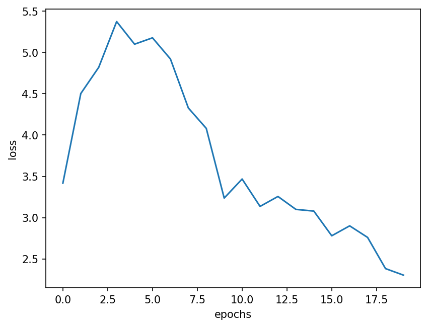
Recurrent Neural Networks (RNN)

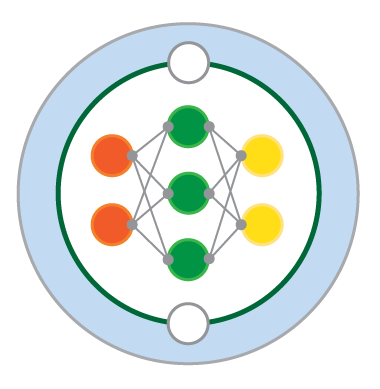
#What is RNN? > Recurrent Neural Network. The hidden state (hidden layer) is used in the next time step. Useful in operations which involve recurrence. In the image below, \(x_t\) is the vector of \(X\) and \(o_t\) is the vector of tendency terms. The network uses \(x_t\) and hidden state \(s_{t-1}\) as inputs to obtain the tendency term \(o_t\). A normal fully connected ANN will only use \(x_t\) to obtain \(o_t\) but RNN uses \(s_{t-1}\) in addition to \(x_t\) to get the output, \(o_t\).

### Applying RNN to L96 model:

# preparing data for training

x1 = torch.Tensor(X_true)  # xk's w.r.t to time
x2 = torch.Tensor(xy_true)  # tendency terms


class L96_RNN(nn.Module):
    def __init__(self, in_n, hid, out_n):
        super(L96_RNN, self).__init__()
        self.h_size = hid
        self.linear1 = nn.Linear(
            in_n + hid, hid
        )  # note that X_k + hidden state is the input
        self.linear2 = nn.Linear(hid, out_n)

    def forward(self, x, hidden):
        # forward code for RNN is different than ANN. Hidden state is also given as input to forward function
        x2 = self.linear1(torch.cat((x, hidden), 1))  # input layer to 1st layer
        x3 = torch.relu(
            x2
        )  # x2 is the hidden state which will be used as input in the next iteration
        x4 = self.linear2(x3)  # x4 is the output layer, tendency terms in L96 case.

        return (
            x4,
            x3,
        )  # x4 is the output layer, and x3 is the hidden layer returned for using in the next iteration

### deletes the model if it already exists
try:
    del model
except:
    pass
###


m = 1  # no. of time steps to use in RNN. untested, code might break if changed.

in_n, hid, out_n = (
    8,
    8,
    8,
)  # X_k, k=1 to 8 and corresponding tendency terms. hid layer nodes can be chaned

model = L96_RNN(in_n, hid, out_n)  # model initialize

l_r = 1e-03  # learning rate

optimizer = torch.optim.Adam(model.parameters(), lr=l_r)  # using Adam optimiser
loss_fn = torch.nn.MSELoss(reduction="mean")  # loss function

epochs = 20  # epochs

loss_array = np.zeros([epochs, 2])  # to store loss for plotting purposes

for p in range(epochs):
    for i in range(time_steps - 1):
        hidd = Variable(torch.randn((1, model.h_size)))
        inp = x1[i : i + m, :].reshape([1, 8])
        outp = x2[i : i + m, :].reshape([1, 8])
        pred, hidd = model.forward(inp, hidd)
        loss = loss_fn(pred, outp)
        # loss.backward()
        model.zero_grad()
        optimizer.zero_grad()
        loss.backward()
        # loss.backward(retain_graph=True)
        optimizer.step()

    loss_array[p, 0] = p
    loss_array[p, 1] = loss.detach().numpy()
    # print('epoch no. >',p, 'loss >',loss.detach().numpy())
plt.figure(dpi=150)
plt.plot(loss_array[:, 1])
plt.ylabel("loss")
plt.xlabel("epochs")
plt.show();

# checking tendency term output from L96 RNN:

hidd = Variable(
    torch.randn((1, model.h_size))
)  # hidden state needs to be initialized for the 1st iteration

pred = torch.zeros([time_steps, 8])  # tendency prediction

for j in range(time_steps - 1):
    inp = x1[j : j + m, :].reshape([1, 8])
    pred[j, :], hidd = model.forward(inp, hidd)

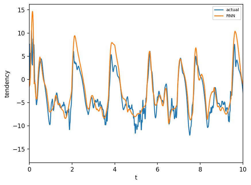
l = 1  # k value. l=k. l goes from 1 to 8 for this example
plt.figure(dpi=150)
plt.plot(t, x2[:, l], "-", label="actual")
plt.plot(t[0:-1], pred[:, l].detach().numpy(), "-", label="RNN")
plt.xlim([0, 10])  # looking only till t=10
plt.legend(fontsize=7)
plt.xlabel("t")
plt.ylabel("tendency")
plt.show();