Random Forest

In this notebook we present some basic application of random forest to the parameterization of the L96 model previously introduced.

import L96_model
import matplotlib.pyplot as plt
import numpy as np
from sklearn import tree
from sklearn.ensemble import RandomForestRegressor, GradientBoostingRegressor
from sklearn.model_selection import train_test_split
from collections import deque
from sklearn.model_selection import RandomizedSearchCV
from L96_model import RK4, L96_eq1_xdot

import torch
import torch.nn as nn
import torch.nn.functional as FF

# Main script parameters
K = 8
J = 32
FORCING = 18
dt = 0.01
T_SPINUP = 50
T_SIMULATIONS = 200

model = L96_model.L96(K, J, F=FORCING)
# First run for spin up
model.run(dt, T_SPINUP, store=True)
# The data from the run below will be used both for offline training and testing
X_history, Y_history, t, closure = model.run(
    dt, T_SIMULATIONS, store=True, return_coupling=True
)

# We will use the quantity below in our online test
var_X = X_history.var()
var_X

20.59244301196517

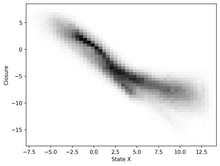
Scatter-plot of subgrid tendency vs large-scale state X

plt.figure(dpi=150)
_ = plt.hist2d(X_history.flatten(), closure.flatten(), bins=50, cmap="binary")
plt.xlabel("State X")
plt.ylabel("Closure")
plt.show();

Starting with a single regression tree

We start with a very simple approach: we use a single value of the state as our feature (i.e. our feature is a scalar), and the subgrid tendency for the same large-scale variable as the target.

Offline training / fitting and testing

closure.shape, X_history.shape

((20001, 8), (20001, 8))

First we split the data into training and test. Since the relation between \(X_k\) and its associated subgrid tendency is not expected to depend on \(k\), we transform the recorded history into a column vector before splitting.

X_train, X_test, xy_train, xy_test = train_test_split(
    X_history.flatten().reshape(-1, 1), closure.flatten(), test_size=0.33, shuffle=False
)

print(f"X_train has shape: {X_train.shape}")
print(f"xy_train has shape: {xy_train.shape}")

X_train has shape: (107205, 1)
xy_train has shape: (107205,)

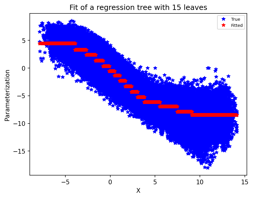
Then we define our decision tree. For the sake of the example, we limit the number of leaves to 15. Feel free to increase that number and see how the plot below, showing the true and fitted data, changes. In particular, for larger values, we can see that we overfit the data.

single_tree = tree.DecisionTreeRegressor(max_leaf_nodes=15)
single_tree.fit(X_train, xy_train)

DecisionTreeRegressor(max_leaf_nodes=15)

In a Jupyter environment, please rerun this cell to show the HTML representation or trust the notebook.
On GitHub, the HTML representation is unable to render, please try loading this page with nbviewer.org.

Here we plot the true training data (the large scale state values on the x-axis, and the parameterization value on the y-axis) and the fitted data.

plt.figure(dpi=150)
plt.plot(X_train, xy_train, "b*")
plt.plot(X_train, single_tree.predict(X_train), "r*")
plt.xlabel("X")
plt.ylabel("Parameterization")
plt.legend(("True", "Fitted"), fontsize=7)
plt.title("Fit of a regression tree with 15 leaves")
plt.show();

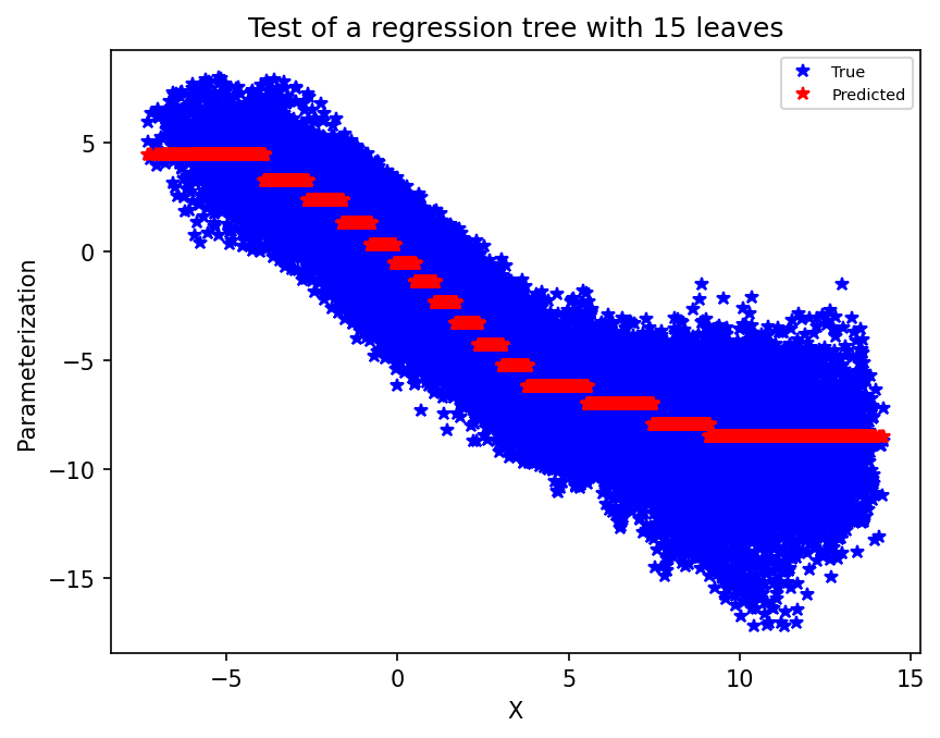
Now, same plot but for the test data. The test data has not been seen during the fitting procedure, so in some sense this is the true test. While we may fit very well the training data, overfitting will result in poor performance on the test dataset.

plt.figure(dpi=150)
plt.plot(X_test, xy_test, "b*")
plt.plot(X_test, single_tree.predict(X_test), "r*")
plt.xlabel("X")
plt.ylabel("Parameterization")
plt.legend(("True", "Predicted"), fontsize=7)
plt.title("Test of a regression tree with 15 leaves")
plt.show();

Fit and test scores

We can compute the \(R^2\) score for both the training data (fit score) and test data.

\[\begin{equation*} R^2 = 1 - \frac{\sum_{i}{(\hat{S}_i - S_i)^2}}{\sum_{i}{(S_i - S_\text{mean})^2}} \end{equation*}\]

fit_score = single_tree.score(X_train, xy_train)
test_score = single_tree.score(X_test, xy_test)

print(fit_score, test_score)

0.8578698255126356 0.8556572030237476

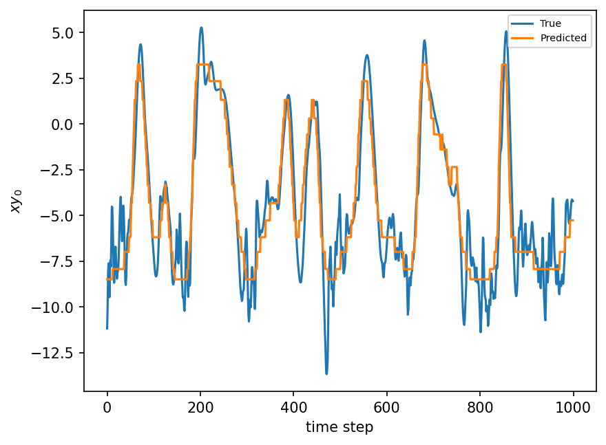
plt.figure(dpi=150)
plt.plot(xy_test[:8000:K])
plt.plot(single_tree.predict(X_test)[:8000:K])
plt.xlabel("time step")
plt.ylabel(r"$xy_0$")
plt.legend(("True", "Predicted"), fontsize=7)
plt.show();

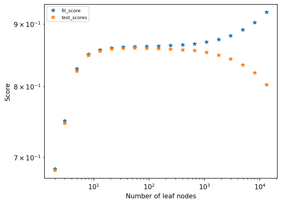
Overfitting

To illustrate what is meant by overfitting, we will increase the number of leaves, and store the fit loss and test loss for plotting

nb_leaves = list(map(lambda x: int(np.exp(x / 2)) + 1, range(1, 20)))

fit_scores, test_scores = [], []
for nb in nb_leaves:
    current_tree = tree.DecisionTreeRegressor(max_leaf_nodes=nb)
    current_tree.fit(X_train, xy_train)
    fit_scores.append(current_tree.score(X_train, xy_train))
    test_scores.append(current_tree.score(X_test, xy_test))

plt.figure(dpi=150)
plt.loglog(nb_leaves, list(fit_scores), "*")
plt.loglog(nb_leaves, list(test_scores), "*")
plt.legend(("fit_score", "test_scores"), fontsize=7)
plt.xlabel("Number of leaf nodes")
plt.ylabel("Score")
plt.show();

Online implementation of the parameterization

Now let’s implement this as a parameterization for L96.

class Parameterization:
    def __init__(self, predictor):
        self.predictor = predictor

    def __call__(self, X):
        X = X.reshape(-1, 1)
        return self.predictor.predict(X)

Here we use the GCM class defined by Yani in his notebook

class GCM:
    def __init__(self, F, parameterization, time_stepping=RK4):
        """
        GCM with paramerization
        Args:
            F: forcing
            parameterization: function that takes parameters and returns a tendency
            time_stepping: time stepping method
        """
        self.F = F
        self.parameterization = parameterization
        self.time_stepping = time_stepping

    def rhs(self, X):
        """
        Args:
            X: state vector
        """
        return L96_eq1_xdot(X, self.F) + self.parameterization(X)

    def __call__(self, X0, dt, nt):
        """
        Args:
            X0: initial conditions
            dt: time increment
            nt: number of forward steps to take
            param: parameters of our closure
        """
        time, hist, X = (
            dt * np.arange(nt + 1),
            np.zeros((nt + 1, len(X0))) * np.nan,
            X0.copy(),
        )
        hist[0] = X

        for n in range(nt):
            X = self.time_stepping(self.rhs, dt, X)
            hist[n + 1], time[n + 1] = X, dt * (n + 1)
        return hist, time

gcm = GCM(model.F, Parameterization(single_tree))
gcm_no_param = GCM(model.F, lambda x: 0)

n_steps = 2000

def online_test(param, n_runs, n_steps):
    simulations = []
    gcm = GCM(model.F, param)
    for i in range(n_runs):
        if i % 10 == 0:
            print("run ", i)
        X_param, t = gcm(model.X, model.dt, n_steps)
        X_no_param, t = gcm_no_param(model.X, model.dt, n_steps)
        X_true, _, _ = model.run(model.dt, n_steps * model.dt, store=True)
        simulations.append((X_true, X_param))
    squared_errors = np.stack(
        [((true - sim) ** 2).mean(axis=-1) for true, sim in simulations], axis=0
    )
    return np.median(squared_errors, axis=0) / var_X

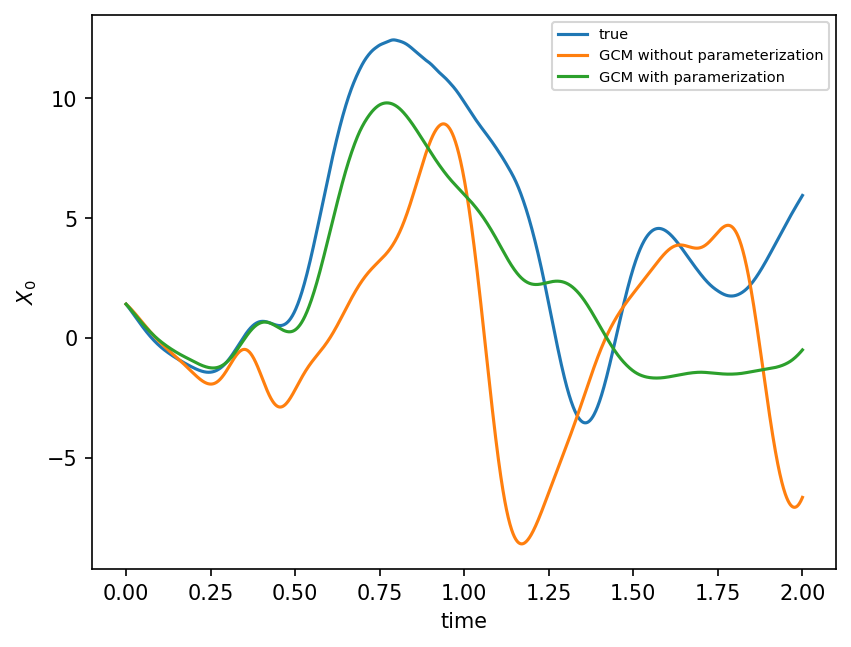
gcm = GCM(model.F, Parameterization(single_tree))
gcm_no_param = GCM(model.F, lambda x: 0)
X_param, t = gcm(model.X, model.dt, n_steps)
X_no_param, t = gcm_no_param(model.X, model.dt, n_steps)
X_true, _, _ = model.run(model.dt, n_steps * model.dt, store=True)

plt.figure(dpi=150)
plt.plot(t, X_true[:, 0], label="true")
plt.plot(t, X_no_param[:, 0], label="GCM without parameterization")
plt.plot(t, X_param[:, 0], label="GCM with paramerization")
plt.xlabel("time")
plt.ylabel(r"$X_0$")
plt.legend(fontsize=7)
plt.show();

Multiple features

In this section, we use the global state.

single_treeV2 = tree.DecisionTreeRegressor(max_leaf_nodes=300)

X_train, X_test, xy_train, xy_test = train_test_split(
    X_history, closure[:, 0], test_size=0.33, shuffle=False
)

single_treeV2.fit(X_train, xy_train)

DecisionTreeRegressor(max_leaf_nodes=300)

In a Jupyter environment, please rerun this cell to show the HTML representation or trust the notebook.
On GitHub, the HTML representation is unable to render, please try loading this page with nbviewer.org.

single_treeV2.score(X_train, xy_train)

0.9411829352805886

single_treeV2.score(X_test, xy_test)

0.8647302377686431

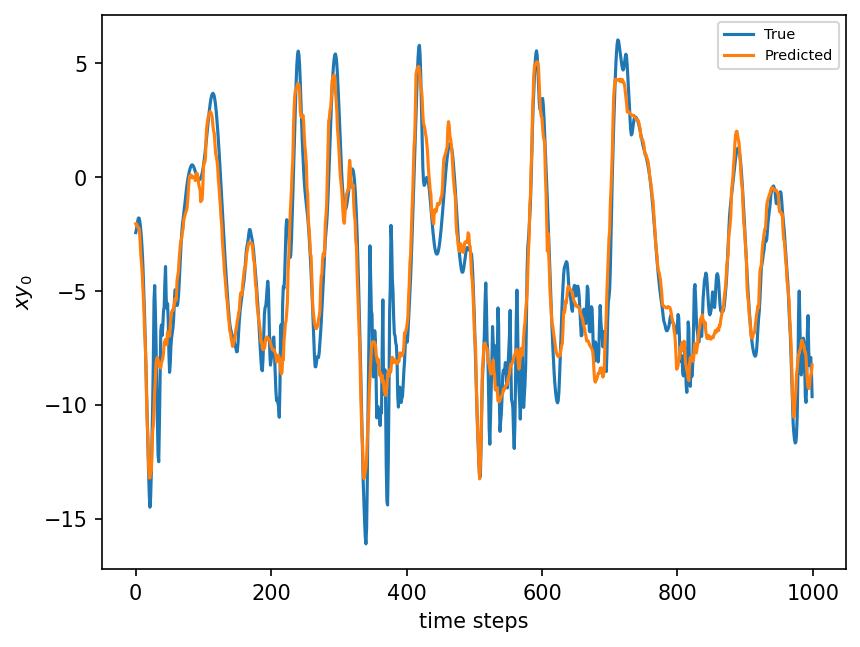
plt.figure(dpi=150)
plt.plot(xy_test[:1000])
plt.plot(single_treeV2.predict(X_test)[:1000])
plt.xlabel("time steps")
plt.ylabel(r"$xy_0$")
plt.legend(("True", "Predicted"), fontsize=7)
plt.show();

We need to adapt our parameterization so that it makes use of the homogeneity of the problem

class ParameterizationV2:
    def __init__(self, predictor):
        self.predictor = predictor

    def __call__(self, X):
        X = X.reshape(1, K)
        new_X = []
        for i in range(K):
            new_X.append(np.roll(X, -i, axis=-1))
        new_X = np.concatenate(new_X, axis=0)
        return self.predictor.predict(new_X)

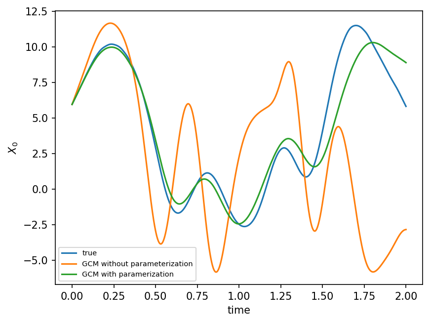
gcm = GCM(model.F, ParameterizationV2(single_treeV2))
gcm_no_param = GCM(model.F, lambda x: 0)
X_param, t = gcm(model.X, model.dt, n_steps)
X_no_param, t = gcm_no_param(model.X, model.dt, n_steps)
X_true, _, _ = model.run(model.dt, n_steps * model.dt, store=True)

plt.figure(dpi=150)
plt.plot(t, X_true[:, 0], label="true")
plt.plot(t, X_no_param[:, 0], label="GCM without parameterization")
plt.plot(t, X_param[:, 0], label="GCM with paramerization")
plt.legend(fontsize=7)
plt.xlabel("time")
plt.ylabel(r"$X_0$")
plt.show();

Random Forest: ensemble of decision trees

Here we use a random forest instead of a single decision tree. The idea is simple: to avoid overfitting, one trains several decision trees on the same data. The prediction of the random forest is then the average prediction of all decision trees within the ensemble.

There are two main ways in which the fitted trees within the forest might differ:

• the selected features for the splits: at each iteration of the fitting procedure, the algorithm does not consider all features to select the best split, at least not when the number of features is large. Instead, a finite number of features is considered at random.

• the data on which they are trained. Below, by setting bootstrap to True and max_samples to 0.5, we specify that each tree within the forest will only be trained on half of the training data

Random forest are an efficient way to avoid overfitting compared to using a single tree. However they do come with a computational and memory cost.

# We start with an ensemble of 10 decision trees
rf = RandomForestRegressor(
    n_estimators=50, max_leaf_nodes=300, bootstrap=True, max_samples=0.5
)

We fit to the same training data as in the previous section

rf.fit(X_train, xy_train)

RandomForestRegressor(max_leaf_nodes=300, max_samples=0.5, n_estimators=50)

In a Jupyter environment, please rerun this cell to show the HTML representation or trust the notebook.
On GitHub, the HTML representation is unable to render, please try loading this page with nbviewer.org.

We can actually get the prediction of each tree within the forest:

tree_predictions = []
for est in rf.estimators_:
    tree_predictions.append(est.predict(X_test[:1, :]))
tree_predictions = np.array(tree_predictions)

print(f"tree_predictions = {tree_predictions.flatten()}")
print(f"mean of tree_predictions = {tree_predictions.mean()}")
print(f"prediction on first row = {rf.predict(X_test[:1, :])[0]}")

tree_predictions = [-5.68866573 -6.36918997 -6.68068083 -6.70684951 -5.88498488 -5.34633724
 -6.80197448 -7.50869645 -7.96469598 -6.79696957 -6.20163157 -6.89236114
 -6.54374019 -7.36572419 -9.59155889 -6.61722669 -6.37638751 -6.70532874
 -5.0823309  -6.925424   -7.25777464 -5.79881966 -6.3427878  -6.85116307
 -7.38335696 -6.80798833 -9.06075126 -7.65073487 -7.33294537 -7.07590675
 -7.27624391 -6.40819231 -6.84209278 -7.1603111  -8.84837085 -7.41667257
 -6.81150927 -6.26821335 -6.56639531 -7.34049438 -6.72380571 -6.92601027
 -6.42858405 -8.18000288 -6.93611799 -6.29285639 -7.49903669 -6.91283743
 -5.45151939 -6.41846482]
mean of tree_predictions = -6.886414372176522
prediction on first row = -6.886414372176523

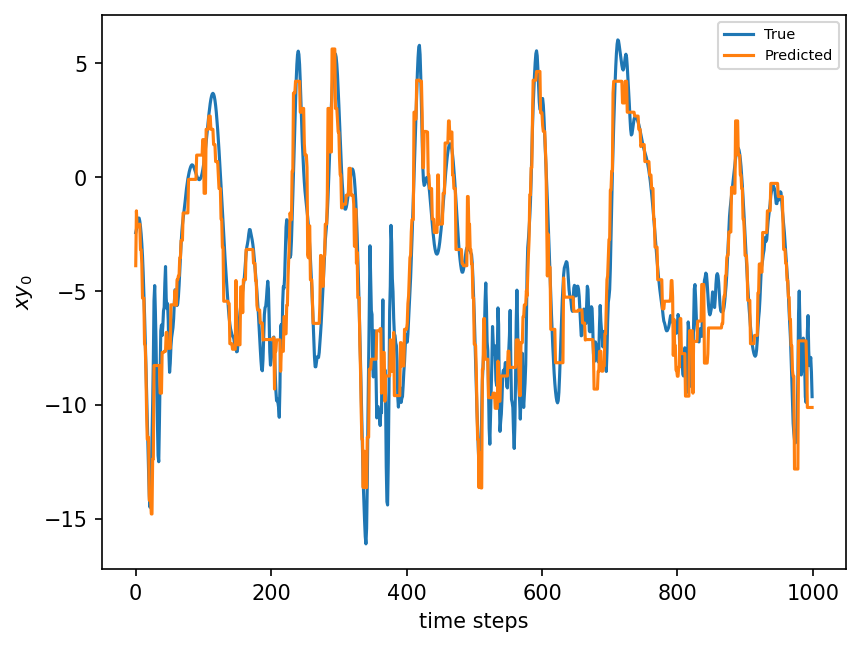
rf.score(X_train, xy_train), rf.score(X_test, xy_test)

(0.9557754806014994, 0.9002932702447579)

plt.figure(dpi=150)
plt.plot(xy_test[:1000])
plt.plot(rf.predict(X_test)[:1000])
plt.xlabel("time steps")
plt.ylabel(r"$xy_0$")
plt.legend(("True", "Predicted"), fontsize=7)
plt.show();

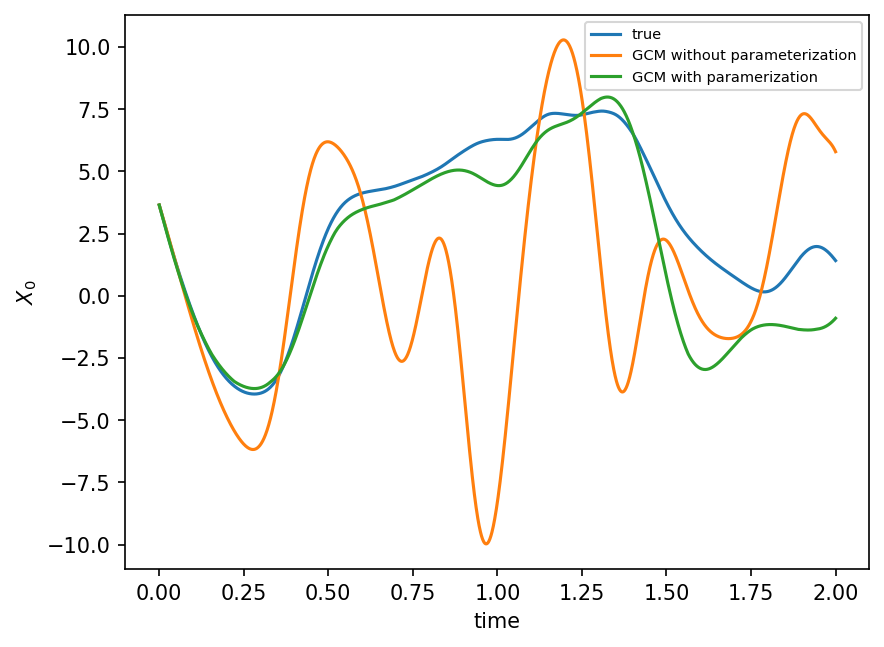
Again, we can test this online.

gcm = GCM(model.F, ParameterizationV2(rf))
gcm_no_param = GCM(model.F, lambda x: 0)

X_param, t = gcm(model.X, model.dt, n_steps)
X_no_param, t = gcm_no_param(model.X, model.dt, n_steps)
X_true, _, _ = model.run(model.dt, n_steps * model.dt, store=True)

plt.figure(dpi=150)
plt.plot(t, X_true[:, 0], label="true")
plt.plot(t, X_no_param[:, 0], label="GCM without parameterization")
plt.plot(t, X_param[:, 0], label="GCM with paramerization")
plt.legend(fontsize=7)
plt.xlabel("time")
plt.ylabel(r"$X_0$")
plt.show();

Gradient boosting

Gradient boosting is a type of machine learning boosting. It relies on the intuition that the best possible next model, when combined with previous models, minimizes the overall prediction error. The key idea is to set the target outcomes for this next model in order to minimize the error.

Further reading here.

gbr = GradientBoostingRegressor(n_estimators=200)
gbr.fit(X_train, xy_train)
score_train = gbr.score(X_train, xy_train)
score_test = gbr.score(X_test, xy_test)

print(score_train, score_test)

0.9230315915543138 0.8899938574149142

More features: using past state

Here we further increase the complexity of our approach by incorporating past state into the features used to carry out our prediction.

n_times = 2
new_X = X_history.copy()
for i in range(n_times - 1):
    new_X = np.concatenate((new_X, np.roll(X_history, i + 1, axis=0)), axis=1)
new_X = new_X[n_times:]
new_closure = closure[n_times:]

X_train, X_test, xy_train, xy_test = train_test_split(
    new_X, new_closure[:, 0], test_size=0.33, shuffle=False
)
X_train.shape

(13399, 16)

rf.max_leaf_nodes = 350
rf.max_samples = 0.99
rf.n_estimators = 100

rf.fit(X_train, xy_train)

RandomForestRegressor(max_leaf_nodes=350, max_samples=0.99)

In a Jupyter environment, please rerun this cell to show the HTML representation or trust the notebook.
On GitHub, the HTML representation is unable to render, please try loading this page with nbviewer.org.

rf.score(X_train, xy_train)

0.9653894936313921

rf.score(X_test, xy_test)

0.9039650671670009

Again we need to adapt the form of the parameterization, here so that it records past values of the state for later use.

class Parameterization:
    def __init__(self, predictor, n_times: int = 5):
        self.predictor = predictor
        self.past_states = deque(maxlen=n_times - 1)
        self.n_times = n_times

    def __call__(self, X):
        X = X.reshape(1, K)
        new_X = []
        for i in range(K):
            new_X.append(np.roll(X, -i, axis=-1))
        new_X = np.concatenate(new_X, 0)
        shape = new_X.shape
        save_X = new_X.copy()
        for i in range(self.n_times - 1):
            try:
                new_X = np.concatenate((new_X, self.past_states[-i - 1]), axis=1)
            except IndexError:
                new_X = np.concatenate((new_X, np.zeros(shape)), axis=-1)
        self.past_states.append(save_X)
        return self.predictor.predict(new_X)

n_steps = 2000
gcm = GCM(model.F, Parameterization(rf, n_times))
gcm_no_param = GCM(model.F, lambda x: 0)
X_param, t = gcm(model.X, model.dt, n_steps)
X_no_param, t = gcm_no_param(model.X, model.dt, n_steps)
X_true, _, _ = model.run(model.dt, n_steps * model.dt, store=True)

plt.figure(dpi=150)
plt.plot(t, X_true[:, 0], label="true")
plt.plot(t, X_no_param[:, 0], label="GCM without parameterization")
plt.plot(t, X_param[:, 0], label="GCM with paramerization")
plt.legend(fontsize=7)
plt.xlabel("time")
plt.ylabel(r"$X_0$")
plt.show();

Comparison with NN parameterization (based on Yani’s code)

class Net_ANN(nn.Module):
    def __init__(self):
        super(Net_ANN, self).__init__()
        self.linear1 = nn.Linear(8, 16)  # 8 inputs, 16 neurons for first hidden layer
        self.linear2 = nn.Linear(16, 16)  # 16 neurons for second hidden layer
        self.linear3 = nn.Linear(16, 8)  # 8 outputs

    def forward(self, x):
        x = FF.relu(self.linear1(x))
        x = FF.relu(self.linear2(x))
        x = self.linear3(x)
        return x

class GCM_network:
    """
    GCM class including a neural network parameterization in rhs of equation for tendency
    Args:
        F: forcing
        parameterization: function that takes parameters and returns a tendency
        time_stepping: time stepping method
    """

    def __init__(self, F, network, time_stepping=RK4):
        self.F = F
        self.network = network
        self.time_stepping = time_stepping

    def rhs(self, X, param=[0]):
        """
        Args:
            X: state vector
            param: parameters of our closure, unused here but maintained for consistency of interface
        """
        if self.network.linear1.in_features == 1:
            X_torch = torch.from_numpy(X).double()
            X_torch = torch.unsqueeze(X_torch, 1)
        else:
            X_torch = torch.from_numpy(np.expand_dims(X, 0)).double()
        return L96_eq1_xdot(X, self.F) + np.squeeze(
            self.network(X_torch).data.numpy()
        )  # Adding NN parameterization

    def __call__(self, X0, dt, nt, param=[0]):
        """
        Args:
            X0: initial conditions
            dt: time increment
            nt: number of forward steps to take
            param: parameters of our closure
        """
        time, hist, X = (
            dt * np.arange(nt + 1),
            np.zeros((nt + 1, len(X0))) * np.nan,
            X0.copy(),
        )
        hist[0] = X

        for n in range(nt):
            X = self.time_stepping(self.rhs, dt, X, param)
            hist[n + 1], time[n + 1] = X, dt * (n + 1)
        return hist, time

# Load network
path_load = "networks/network_3_layers_100_epoches.pth"
nn_3l = Net_ANN().double()
nn_3l.load_state_dict(torch.load(path_load))

<All keys matched successfully>

n_steps = 2000
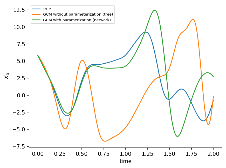
gcm = GCM(model.F, ParameterizationV2(single_treeV2))
gcm_network = GCM_network(model.F, nn_3l)
X_param, t = gcm(model.X, model.dt, n_steps)
X_network, t = gcm_network(model.X, model.dt, n_steps)
X_no_param, t = gcm_no_param(model.X, model.dt, n_steps)
X_true, _, _ = model.run(model.dt, n_steps * model.dt, store=True)

plt.figure(dpi=150)
plt.plot(t, X_true[:, 0], label="true")
plt.plot(t, X_no_param[:, 0], label="GCM without parameterization (tree)")
plt.plot(t, X_param[:, 0], label="GCM with paramerization (network)")
plt.legend(fontsize=7)
plt.xlabel("time")
plt.ylabel(r"$X_0$")
plt.show();

Which model / model parameters should we go for?

Standard Machine Learning approach: validation

The Machine Learning approach to this problem is to separate the data into three data sets:

• training dataset

• validation dataset

• test dataset

Only data from the training dataset is used for fitting. The validation dataset is then used for model selection and hyperparameters tuning: we select the model whose performance on the validation dataset is best.

In order to choose hyperparameters, one needs to make a decision on what set of values to try. One approach is to try a grid of values. Another approach is to try random values. This is recommanded when the possible number of hyperparameter combinations is large. Finally Bayesian approaches to this problem are also popular. Further reading on grid search, random search and bayesian approach here.

Here we shall implement the random approach: for each model, we will define a range of values for each parameter we wish to tune. We will randomly select a combination of parameter values, fit the model to the training dataset, and assess its performance on the validation dataset. The combination of values leading to the best validation score will be retained.

single_tree_params_dist = {
    "max_leaf_nodes": list(map(int, 1 + np.exp(np.arange(11)))),
}

rf_params_dist = {
    "max_leaf_nodes": list(map(int, 1 + np.exp(np.arange(13)))),
    "n_estimators": np.arange(1, 10) * 50,
}

X_train, X_test, xy_train, xy_test = train_test_split(
    X_history, closure[:, 0], test_size=0.33
)

The cells below are very slow to execute. Uncomment them to perform the parameter search.

# best_single_treeV2 = RandomizedSearchCV(
#     single_treeV2, single_tree_params_dist, n_iter=10, verbose=True
# )
# best_rf = RandomizedSearchCV(rf, rf_params_dist, n_iter=20, verbose=True)

# best_single_treeV2.fit(X_train, xy_train)
# best_rf.fit(X_train, xy_train)

# print("single tree")
# print(f"best score = {best_single_treeV2.best_score_}")
# print(f"best parameters = {best_single_treeV2.best_params_}")
# print("\nrandom forest")
# print(f"best score = {best_rf.best_params_}")
# print(f"best parameters = {best_rf.score(X_test, xy_test)}")