Learning Data Assimilation Increments#
This notebook is derived from the previous notebooks: Neural_network_for_Lorenz96 and Data Assimilation demo in the Lorenz 96 (L96) two time-scale model.
We’ve restricted it to only using the 3-layer network (not the linear regression model)
import time

import matplotlib.pyplot as plt
import numpy as np
import torch
from torch import nn
from torch.optim import Adam
from torch.utils.data import DataLoader, TensorDataset

import DA_methods
from L96_model import L96, L96_eq1_xdot
# Ensuring reproducibility
rng = np.random.default_rng()
torch.manual_seed(42);
Defining the Model, its Parameters, and Other Utility Functions#
Defining the General Circulation Model (GCM)#
def GCM(X_init, F, dt, nt, param=[0]):
    """A toy `General Circulation Model` (GCM) that uses the single
    time-scale Lorenz 1996 model with a parameterised coupling term
    to represent the interaction between the observed coarse scale
    processes `X` and unobserved fine scale processes `Y` of the two
    time-scale model.

    Args:
        X_init: Initial conditions of X
        F: Forcing term
        dt: Sampling frequency of the model
        nt: Number of timesteps for which to run the model
        param: Weights to give to the coupling term

    Returns:
        Model output for all variables of X at each timestep along with
        the corresponding time units
    """
    time, hist, X = (
        dt * np.arange(nt + 1),
        np.zeros((nt + 1, len(X_init))) * np.nan,
        X_init.copy(),
    )
    hist[0] = X

    for n in range(nt):
        X = X + dt * (L96_eq1_xdot(X, F) - np.polyval(param, X))
        hist[n + 1], time[n + 1] = X, dt * (n + 1)

    return hist, time
Defining the Utility Functions#
def s(k, K):
    """A non-dimension coordinate from -1..+1 corresponding to k=0..K"""
    return 2 * (0.5 + k) / K - 1
def get_dist(i, j, K):
    """Compute the absolute distance between two element indices
    within a square matrix of size (K x K)

    Args:
        i: the ith row index
        j: the jth column index
        K: shape of square array

    Returns:
        Distance
    """
    return abs(i - j) if abs(i - j) <= 0.5 * K / 2 else K - abs(i - j)
def observation_operator(K, l_obs, t_obs, i_t):
    """Observation operator to map between model and observation space,
    assuming linearity and model space observations.

    Args:
        K: spatial dimension of the model
        l_obs: spatial positions of observations on model grid
        t_obs: time positions of observations
        i_t: the timestep of the current DA cycle

    Returns:
        Operator matrix (K * observation_density, K)
    """
    n = l_obs.shape[-1]
    H = np.zeros((n, K))
    H[range(n), l_obs[t_obs == i_t]] = 1
    return H
def gaspari_cohn(distance, radius):
    """Compute the appropriate distance dependent weighting of a
    covariance matrix, after Gaspari & Cohn, 1999 (https://doi.org/10.1002/qj.49712555417)

    Args:
        distance: the distance between array elements
        radius: localization radius for DA

    Returns:
        distance dependent weight of the (i,j) index of a covariance matrix
    """
    if distance == 0:
        weight = 1.0
    else:
        if radius == 0:
            weight = 0.0
        else:
            ratio = distance / radius
            weight = 0.0
            if ratio <= 1:
                weight = (
                    -(ratio**5) / 4
                    + ratio**4 / 2
                    + 5 * ratio**3 / 8
                    - 5 * ratio**2 / 3
                    + 1
                )
            elif ratio <= 2:
                weight = (
                    ratio**5 / 12
                    - ratio**4 / 2
                    + 5 * ratio**3 / 8
                    + 5 * ratio**2 / 3
                    - 5 * ratio
                    + 4
                    - 2 / 3 / ratio
                )
    return weight
def localize_covariance(B, loc=0):
    """Localize the model climatology covariance matrix, based on
    the Gaspari-Cohn function.

    Args:
        B: Covariance matrix over a long model run 'M_truth' (K, K)
        loc: spatial localization radius for DA

    Returns:
        Covariance matrix scaled to zero outside distance 'loc' from diagonal and
        the matrix of weights which are used to scale covariance matrix
    """
    M, N = B.shape
    X, Y = np.ix_(np.arange(M), np.arange(N))
    dist = np.vectorize(get_dist)(X, Y, M)
    W = np.vectorize(gaspari_cohn)(dist, loc)
    return B * W, W
def running_average(X, N):
    """Compute running mean over a user-specified window.

    Args:
        X: Input vector of arbitrary length 'n'
        N: Size of window over which to compute mean

    Returns:
        X averaged over window N
    """
    if N % 2 == 0:
        N1, N2 = -N / 2, N / 2
    else:
        N1, N2 = -(N - 1) / 2, (N + 1) / 2
    X_sum = np.zeros(X.shape)
    for i in np.arange(N1, N2):
        X_sum = X_sum + np.roll(X, int(i), axis=0)
    return X_sum / N
def find_obs(loc, obs, t_obs, l_obs, period):
    """NOTE: This function is for plotting purposes only."""
    t_period = np.where((t_obs[:, 0] >= period[0]) & (t_obs[:, 0] < period[1]))
    obs_period = np.zeros(t_period[0].shape)
    obs_period[:] = np.nan
    for i in np.arange(len(obs_period)):
        if np.any(l_obs[t_period[0][i]] == loc):
            obs_period[i] = obs[t_period[0][i]][l_obs[t_period[0][i]] == loc]
    return obs_period
Initializing the Lorenz 1996 Model Parameters#
Let’s define the parameters of the Lorenz 1996 model that match those of Wilks, 2005; K=8, J=32, F=18.
class Config:
    # fmt: off
    K = 8                               # Dimension of L96 `X` variables
    J = 32                              # Dimension of L96 `Y` variables
    obs_freq = 10                       # Observation frequency (number of sampling intervals (si) per observation)
    F_truth = 18                        # F for truth signal
    F_fcst = 18                         # F for forecast (DA) model
    GCM_param = np.array([0, 0, 0, 0])  # Polynomial coefficicents for GCM parameterization
    ns_da = 4000                        # Number of time samples for DA
    ns = 4000                           # Number of time samples for truth signal
    ns_spinup = 200                     # Number of time samples for spin up
    dt = 0.005                          # Model timestep
    si = 0.005                          # Truth sampling interval
    B_loc = 0.0                         # Spatial localization radius for DA
    DA = "EnKF"                         # DA method
    nens = 50                           # Number of ensemble members for DA
    inflate_opt = "relaxation"          # Method for DA model covariance inflation
    inflate_factor = 0.86               # Inflation factor
    obs_density = 1.0                   # Fraction of spatial gridpoints where observations are collected
    DA_freq = 10                        # Assimilation frequency (number of sampling intervals (si) per assimilation step)
    obs_sigma = 0.1                     # Observational error standard deviation
    initial_spread = 0.1                # Initial spread added to initial conditions
    # fmt: on
Suggestions for Modifying the L96 Model Paramters#
If you want to modify the default model parameters given above, you can use the suggestions below for alternate values depending upon the desired behaviour.
Less certain observations
obs_sigma: 1.0initial_spread: 1.0inflate_factor: 0.5
Less frequent observations
obs_freq: 50DA_freq: 50inflate_factor: 0.4
Very infrequent observations
obs_freq: 200DA_freq: 200inflate_factor: 0.5
More frequent observations
obs_freq: 5DA_freq: 5inflate_factor: 0.9
Very frequent observations
obs_freq: 1DA_freq: 1inflate_factor: 0.98
Very frequent observations but less accurate
obs_freq: 1DA_freq: 1obs_sigma: 1.0initial_spread: 1.0inflate_factor: 0.9
Different time-scale
F_fcst: 16
Generate Truth Run from Two Time-Scale L96 Model#
The L96 two time-scale model acts as the real world using which we obtain the unobserved truth field from which our observations will be derived.
We begin by spinning-up a state and then record a series of \(X\) and \(Y\) at time \(t\) in arrays X_truth, Y_truth and t_truth respectively. The initial state \(X(t=0\) is recorded in X_init (and equal to X_truth[0]).
# Set up the "truth" 2-scale L96 model
M_truth = L96(Config.K, Config.J, F=Config.F_truth, dt=Config.dt)
M_truth.set_state(rng.standard_normal((Config.K)), 0 * M_truth.j)

# The model runs for `ns_spinup` timesteps to spin-up
X_spinup, Y_spinup, t_spinup = M_truth.run(Config.si, Config.si * Config.ns_spinup)

# Generate the initial conditions of X and Y
X_init = X_spinup[-1, :]
Y_init = Y_spinup[-1, :]

# Using the initial conditions, generate the truth
M_truth.set_state(X_init, Y_init)
X_truth, Y_truth, t_truth = M_truth.run(Config.si, Config.si * Config.ns)
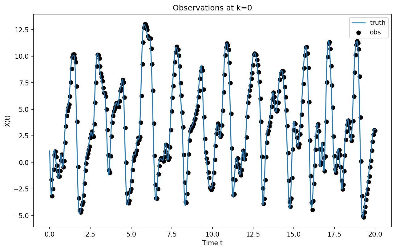
Generate Synthetic Observations#
Now we create some observations of the real world by sampling at obs_freq intervals and adding some noise (observational error).
# Sample the "truth" to generate observations at certain times (t_obs) and locations (l_obs)
t_obs = np.tile(
    np.arange(Config.obs_freq, Config.ns_da + Config.obs_freq, Config.obs_freq),
    [int(Config.K * Config.obs_density), 1],
).T

l_obs = np.zeros(t_obs.shape, dtype="int")
for i in range(l_obs.shape[0]):
    l_obs[i, :] = rng.choice(
        Config.K, int(Config.K * Config.obs_density), replace=False
    )

X_obs = X_truth[t_obs, l_obs] + Config.obs_sigma * rng.standard_normal(l_obs.shape)
# Calculated observation covariance matrix, assuming independent observations
R = Config.obs_sigma**2 * np.eye(int(Config.K * Config.obs_density))
plt.figure(figsize=[10, 6], dpi=150)
plt.plot(t_truth[:], X_truth[:, 0], label="truth")
plt.scatter(
    t_truth[t_obs[1:, 0]],
    find_obs(0, X_obs, t_obs, l_obs, [t_obs[0, 0], t_obs[-1, 0]]),
    color="k",
    label="obs",
)
plt.legend()
plt.xlabel("Time t")
plt.ylabel("X(t)")
plt.title("Observations at k=0");
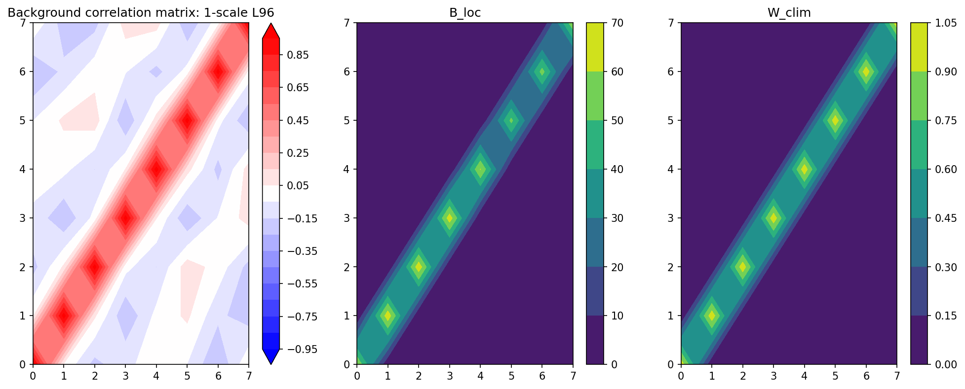
Apply Localization to the Background Model Covariance#
We run the model in forward mode for 5000 steps to calculate the background covariance. The model is the GCM function defined above which integrates forward.
The absence of the coupling term to the \(Y\) equations makes this a model with missing physics that we hope the Ensemble Kalman Filter will correct.
# Generate climatological background covariance for 1-scale L96 model
X1_clim, _ = GCM(X_init, Config.F_fcst, Config.dt, 5000)
B_clim1 = np.cov(X1_clim.T)
# Load pre-calculated climatological background covariance matrix from a long simulation
B_loc, W_clim = localize_covariance(B_clim1, loc=Config.B_loc)

B_corr1 = np.zeros(B_clim1.shape)
for i in range(B_clim1.shape[0]):
    for j in range(B_clim1.shape[1]):
        B_corr1[i, j] = B_clim1[i, j] / np.sqrt(B_clim1[i, i] * B_clim1[j, j])
plt.figure(figsize=(16, 6), dpi=150)
plt.subplot(131)
plt.contourf(B_corr1, cmap="bwr", extend="both", levels=np.linspace(-0.95, 0.95, 20))
plt.colorbar()
plt.title("Background correlation matrix: 1-scale L96")
plt.subplot(132)
plt.contourf(B_loc)
plt.colorbar()
plt.title("B_loc")
plt.subplot(133)
plt.contourf(W_clim)
plt.colorbar()
plt.title("W_clim");
Run Data Assimilation#
The algorithms steps through segments of time (DA cycles), launching an ensemble of short forecasts from the posterior estimate of the preceding segment, each perturbed by noise in their initial condition (inflation).
Each ensemble trajectory is stored in ensX. The increment added to correct the prior is in X_inc.
# Set up array to store DA increments
X_inc = np.zeros((int(Config.ns_da / Config.DA_freq), Config.K, Config.nens))
if Config.DA == "3DVar":
    X_inc = np.squeeze(X_inc)
t_DA = np.zeros(int(Config.ns_da / Config.DA_freq))
# Initialize ensemble with perturbations
i_t = 0
ensX = X_init[None, :, None] + rng.standard_normal((1, Config.K, Config.nens))
X_post = ensX[0, ...]
W = W_clim
for cycle in np.arange(0, Config.ns_da / Config.DA_freq, dtype=int):
    # Set up array to store model forecast for each DA cycle
    ensX_fcst = np.zeros((Config.DA_freq + 1, Config.K, Config.nens))

    # Model forecast for next DA cycle
    for n in range(Config.nens):
        ensX_fcst[..., n] = GCM(
            X_post[0 : Config.K, n],
            Config.F_fcst,
            Config.dt,
            Config.DA_freq,
            Config.GCM_param,
        )[0]

    i_t = i_t + Config.DA_freq

    # Get prior/background from the forecast
    X_prior = ensX_fcst[-1, ...]

    # Call DA
    t_DA[cycle] = t_truth[i_t]
    if Config.DA == "EnKF":
        H = observation_operator(Config.K, l_obs, t_obs, i_t)

        # Augment state vector with parameters when doing parameter estimation
        B_ens = np.cov(X_prior)
        B_ens_loc = B_ens * W[0 : Config.K, 0 : Config.K]
        X_post = DA_methods.EnKF(X_prior, X_obs[t_obs == i_t], H, R, B_ens_loc)
        X_post[0 : Config.K, :] = DA_methods.ens_inflate(
            X_post[0 : Config.K, :],
            X_prior[0 : Config.K, :],
            Config.inflate_opt,
            Config.inflate_factor,
        )
    elif Config.DA == "None":
        X_post = X_prior

    if not Config.DA == "None":
        # Get current increments
        X_inc[cycle, ...] = (
            np.squeeze(X_post[0 : Config.K, ...]) - X_prior[0 : Config.K, ...]
        )

    # Reset initial conditions for next DA cycle
    ensX_fcst[-1, :, :] = X_post[0 : Config.K, :]
    ensX = np.concatenate((ensX, ensX_fcst[1:None, ...]))
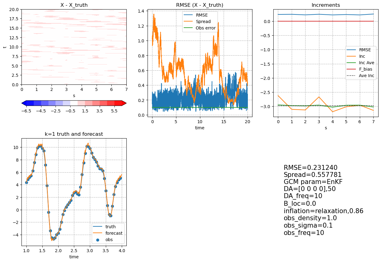
Post Processing and Visualization#
meanX is the ensemble mean forecast, averaging over all the ensemble members. It has discontinuities due to the increment addition between each DA segment.
meanX = np.mean(ensX, axis=-1)
clim = np.max(np.abs(meanX - X_truth[0 : (Config.ns_da + 1), :]))
fig, axes = plt.subplots(2, 3, figsize=(15, 10))
ch = axes[0, 0].contourf(
    M_truth.k,
    t_truth[0 : (Config.ns_da + 1)],
    meanX - X_truth[0 : (Config.ns_da + 1), :],
    cmap="bwr",
    levels=np.arange(-6.5, 7, 1),
    extend="both",
)
plt.colorbar(ch, ax=axes[0, 0], orientation="horizontal")
axes[0, 0].set_xlabel("s")
axes[0, 0].set_ylabel("t")
axes[0, 0].set_title("X - X_truth")
axes[0, 1].plot(
    t_truth[0 : (Config.ns_da + 1)],
    np.sqrt(((meanX - X_truth[0 : (Config.ns_da + 1), :]) ** 2).mean(axis=-1)),
    label="RMSE",
)
axes[0, 1].plot(
    t_truth[0 : (Config.ns_da + 1)],
    np.mean(np.std(ensX, axis=-1), axis=-1),
    label="Spread",
)
axes[0, 1].plot(
    t_truth[0 : (Config.ns_da + 1)],
    Config.obs_sigma * np.ones((Config.ns_da + 1)),
    label="Obs error",
)
axes[0, 1].legend()
axes[0, 1].set_xlabel("time")
axes[0, 1].set_title("RMSE (X - X_truth)")
axes[0, 1].grid(which="both", linestyle="--")

axes[0, 2].plot(
    M_truth.k,
    np.sqrt(((meanX - X_truth[0 : (Config.ns_da + 1), :]) ** 2).mean(axis=0)),
    label="RMSE",
)
X_inc_ave = X_inc / Config.DA_freq / Config.si
axes[0, 2].plot(M_truth.k, X_inc_ave.mean(axis=(0, -1)), label="Inc")
axes[0, 2].plot(
    M_truth.k, running_average(X_inc_ave.mean(axis=(0, -1)), 7), label="Inc Ave"
)
axes[0, 2].plot(
    M_truth.k,
    np.ones(M_truth.k.shape) * (Config.F_fcst - Config.F_truth),
    label="F_bias",
)
axes[0, 2].plot(
    M_truth.k,
    np.ones(M_truth.k.shape) * (X_inc / Config.DA_freq / Config.si).mean(),
    "k:",
    label="Ave Inc",
)
axes[0, 2].legend()
axes[0, 2].set_xlabel("s")
axes[0, 2].set_title("Increments")
axes[0, 2].grid(which="both", linestyle="--")

plot_start, plot_end = 200, 800
plot_start_DA, plot_end_DA = int(plot_start / Config.DA_freq), int(
    plot_end / Config.DA_freq
)
plot_x = 0
axes[1, 0].plot(
    t_truth[plot_start:plot_end], X_truth[plot_start:plot_end, plot_x], label="truth"
)
axes[1, 0].plot(
    t_truth[plot_start:plot_end], meanX[plot_start:plot_end, plot_x], label="forecast"
)
axes[1, 0].scatter(
    t_DA[plot_start_DA - 1 : plot_end_DA - 1],
    find_obs(plot_x, X_obs, t_obs, l_obs, [plot_start, plot_end]),
    label="obs",
)
axes[1, 0].grid(which="both", linestyle="--")
axes[1, 0].set_xlabel("time")
axes[1, 0].set_title("k=" + str(plot_x + 1) + " truth and forecast")
axes[1, 0].legend()

axes[1, 1].axis("off")

axes[1, 2].text(
    0.1,
    0.1,
    "RMSE={:3f}\nSpread={:3f}\nGCM param={}\nDA={},{}\nDA_freq={}\nB_loc={}\ninflation={},{}\nobs_density={}\nobs_sigma={}\nobs_freq={}".format(
        np.sqrt(((meanX - X_truth[0 : (Config.ns_da + 1), :]) ** 2).mean()),
        np.mean(np.std(ensX, axis=-1)),
        Config.DA,
        Config.GCM_param,
        Config.nens,
        Config.DA_freq,
        Config.B_loc,
        Config.inflate_opt,
        Config.inflate_factor,
        Config.obs_density,
        Config.obs_sigma,
        Config.obs_freq,
    ),
    fontsize=15,
)
axes[1, 2].axis("off");
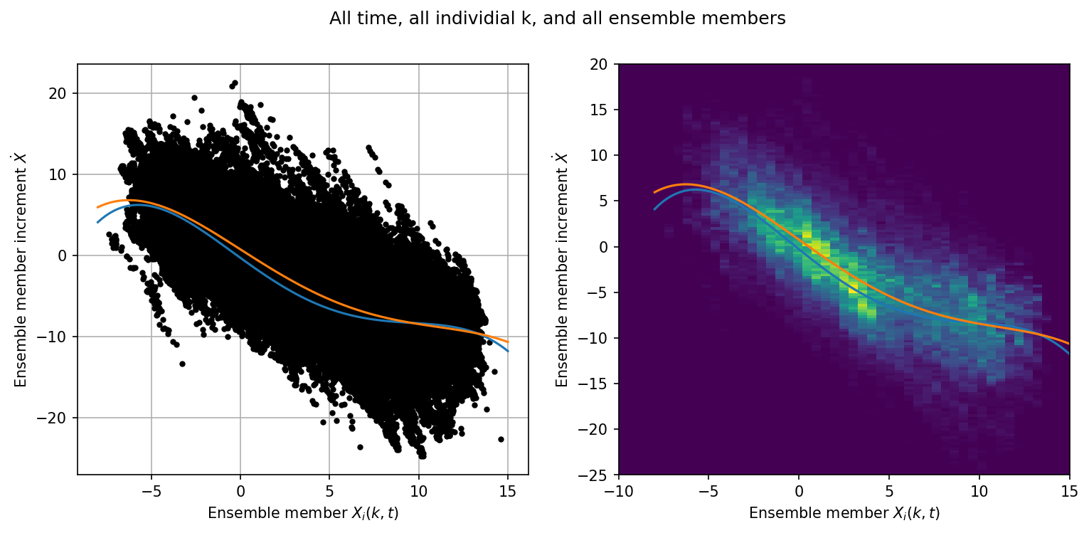
Examining the Relationship between the Members and their Increments#
Converting the increment X_inc into a tendency, we can examine the relationship between \(\dot{X}\) (due to the missing physics) and the state of the model at the beginning of each DA segment.
If we are properly correcting the absence of the coupling term then this structure should look like the parameterization of the coupling term, as done in Wilks, 2005.
Individual Ensemble Members#
jj = np.abs(X_inc_ave[0:, :].flatten()) > -1e-7

# The offset by DA_freq looks at the previous posterior
x_input = ensX[t_obs[0:, 0] - Config.DA_freq, :].flatten()[jj]

# Mid-point of trajectory
x_input = 0.5 * (x_input + ensX[t_obs[0:, 0], :].flatten()[jj])

xinc_output = X_inc_ave[0:, :].flatten()[jj]

x = np.linspace(-8, 15, 100)
p = np.polyfit(x_input, xinc_output, 4)
p18 = [0.000707, -0.0130, -0.0190, 1.59, 0.275]  # Polynomial from Wilks, 2005
plt.figure(figsize=(12, 5), dpi=150)
plt.suptitle("All time, all individial k, and all ensemble members")
plt.subplot(121)
plt.plot(x_input, xinc_output, "k.")
plt.grid()
plt.plot(x, -np.polyval(p18, x), label="$P_4(X_k)$ - Wilks, 2005")
plt.plot(x, np.polyval(p, x), label="$P_4(X_k)$")
plt.xlabel("Ensemble member $X_i(k,t)$")
plt.ylabel("Ensemble member increment $\dot{X}$")
plt.subplot(122)
plt.hist2d(
    x_input, xinc_output, bins=(np.linspace(-10, 15, 50), np.linspace(-25, 20, 150))
)
plt.plot(x, -np.polyval(p18, x), label="$P_4(X_k)$ - Wilks, 2005")
plt.plot(x, np.polyval(p, x), label="$P_4(X_k)$")
plt.xlabel("Ensemble member $X_i(k,t)$")
plt.ylabel("Ensemble member increment $\dot{X}$");
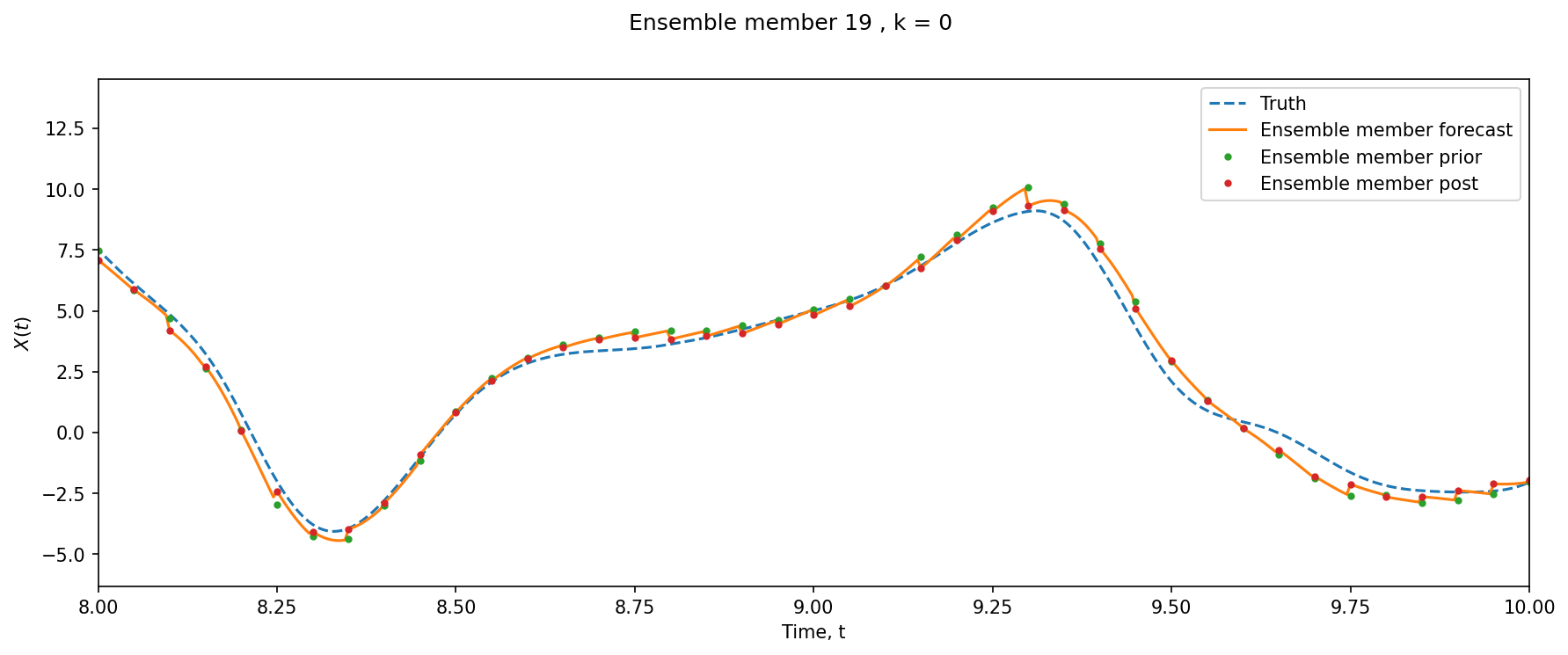
xl = 8, 10
k = 0
e = 19
si = Config.DA_freq

l = (l_obs == k).max(axis=1)

plt.figure(figsize=(14, 5), dpi=150)
plt.suptitle("Ensemble member %i , k = %i" % (e, k))
plt.plot(t_truth, X_truth[:, k], "--", label="Truth")
plt.plot(t_truth, ensX[:, k, e], label="Ensemble member forecast")
plt.plot(
    t_truth[t_obs[l, 0]],
    ensX[si::si, k, e][l] - X_inc[:, :, e][l, k],
    ".",
    label="Ensemble member prior",
)
plt.plot(t_truth[t_obs[l, 0]], ensX[si::si, k, e][l], ".", label="Ensemble member post")
plt.xlim(xl)
plt.xlabel("Time, t")
plt.ylabel("$X(t)$")
plt.legend();
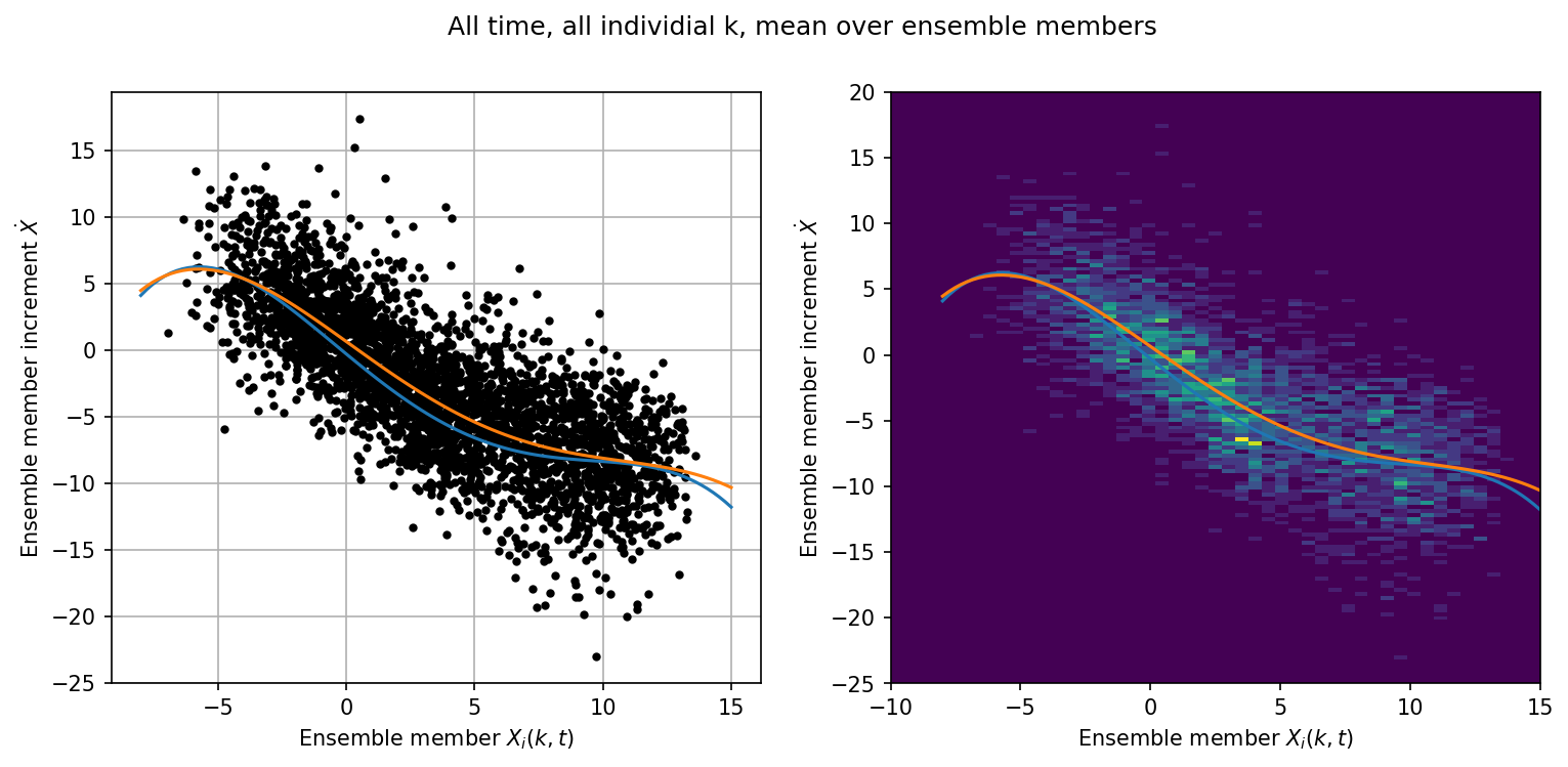
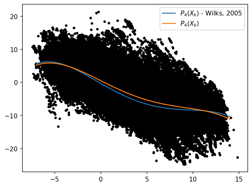
Mean over Ensemble Members#
jj = np.abs(X_inc_ave.mean(axis=-1).flatten()) > -1e-7

# The offset by DA_freq looks at the previous posterior
x_input = meanX[t_obs[0:, 0] - Config.DA_freq].flatten()[jj]

# Mid-point of trajectory
x_input = 0.5 * (x_input + meanX[t_obs[0:, 0]].flatten()[jj])

xinc_output = X_inc_ave.mean(axis=-1).flatten()[jj]

x = np.linspace(-8, 15, 100)
p = np.polyfit(x_input, xinc_output, 4)
p18 = [0.000707, -0.0130, -0.0190, 1.59, 0.275]  # Polynomial from Wilks, 2005
plt.figure(figsize=(12, 5), dpi=150)
plt.suptitle("All time, all individial k, mean over ensemble members")
plt.subplot(121)
plt.plot(x_input, xinc_output, "k.")
plt.grid()
plt.plot(x, -np.polyval(p18, x), label="$P_4(X_k)$ - Wilks, 2005")
plt.plot(x, np.polyval(p, x), label="$P_4(X_k)")
plt.xlabel("Ensemble member $X_i(k,t)$")
plt.ylabel("Ensemble member increment $\dot{X}$")
plt.subplot(122)
plt.hist2d(
    x_input, xinc_output, bins=(np.linspace(-10, 15, 50), np.linspace(-25, 20, 150))
)
plt.plot(x, -np.polyval(p18, x), label="$P_4(X_k)$ - Wilks, 2005")
plt.plot(x, np.polyval(p, x), label="$P_4(X_k)")
plt.xlabel("Ensemble member $X_i(k,t)$")
plt.ylabel("Ensemble member increment $\dot{X}$");
xl = 8, 10
k = 0
si = Config.DA_freq

l = (l_obs == k).max(axis=1)

plt.figure(figsize=(14, 5), dpi=150)
plt.suptitle("Ensemble mean, k = %i" % (k))
plt.plot(t_truth, X_truth[:, k], "--", label="Truth")
plt.fill_between(
    t_truth,
    meanX[:, k] - ensX[:, k, :].std(axis=-1),
    meanX[:, k] + ensX[:, k, :].std(axis=-1),
    color="grey",
    alpha=0.2,
    label="Ensemble spread",
)
plt.plot(t_truth, meanX[:, k], label="Ensemble mean forecast")
plt.plot(
    t_truth[t_obs[l, 0]],
    meanX[si::si, k][l] - X_inc.mean(axis=-1)[l, k],
    ".",
    label="Ensemble mean prior",
)
plt.plot(t_truth[t_obs[l, 0]], meanX[si::si, k][l], ".", label="Ensemble mean post")
plt.xlim(xl)
plt.xlabel("Time, t")
plt.ylabel("$X(t)$")
plt.legend();
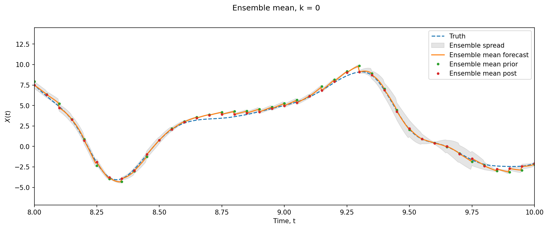
With this, we have successfully created the DA increments.
Learning the DA Increments#
With the dataset for DA Increments created above, we now build a neural network which will try to model that dataset so that we can use it for unseen observations.
t_inc = t_truth[
    t_obs[:, 0]
]  # These are the times in the "real world" when observations were made
dt_inc = np.diff(t_inc)[0]  # Time interval between increments

dt = np.diff(t_truth)[0]  # Time-step of "real world" model
da_interval = int(dt_inc / dt)

# Data from DA system (increments for individual ensemble members)
x_input = ensX[:-1:da_interval]
X_tend = X_inc / dt_inc
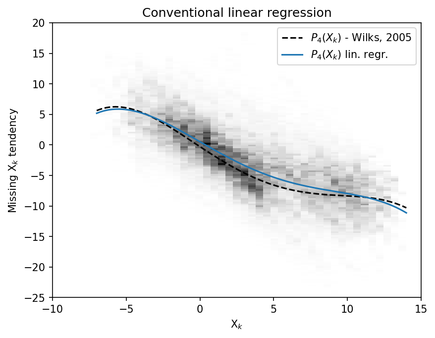
Observing the Dataset#
As a sanity check, we look at the data for obvious structure. A polyfit to the data will compare well to Wilks 2005, if the data is similar in distribution. We show Wilks 2005 and the 4th order polyfit for reference but neither are used or needed for training the neural network.
# A simple scatter plot of x_tend against x_input
x = np.linspace(-7, 14, 100)
p = np.polyfit(x_input.flatten(), X_tend.flatten(), 4)
p18 = [0.000707, -0.0130, -0.0190, 1.59, 0.275]  # Polynomial from Wilks, 2005
plt.figure(dpi=150)
plt.plot(x_input.flatten(), X_tend.flatten(), "k.")
plt.plot(x, -np.polyval(p18, x), label="$P_4(X_k)$ - Wilks, 2005")
plt.plot(x, np.polyval(p, x), label="$P_4(X_k)$")
plt.legend();
# A PDf of x_tend against x_input
plt.figure(dpi=150)
plt.hist2d(
    x_input.flatten(),
    X_tend.flatten(),
    bins=(np.linspace(-10, 15, 50), np.linspace(-25, 20, 150)),
    cmap=plt.cm.Greys,
)
plt.plot(x, -np.polyval(p18, x), "k--", label="$P_4(X_k)$ - Wilks, 2005")
plt.plot(x, np.polyval(p, x), label="$P_4(X_k)$ lin. regr.")
plt.legend()
plt.xlabel("X$_k$")
plt.ylabel("Missing X$_k$ tendency")
plt.title("Conventional linear regression");
Creating the Dataset Split#
We partition the dataset into training (seen by the network during optimization of the weights) and validation (used for evaluation) sets.
train_size = x_input.size // 2
train_size = int(0.7 * x_input.size)
print("Training set size =", train_size, "out of", x_input.size)

# Convert the data to type float32
x_input, X_tend = x_input.astype(np.float32), X_tend.astype(np.float32)

X_train = x_input.flatten()[:train_size]
Y_train = X_tend.flatten()[:train_size]
X_val = x_input.flatten()[train_size:]
Y_val = X_tend.flatten()[train_size:]
Training set size = 112000 out of 160000
Building the Dataset#
BATCH_SIZE = 1024

# Training Dataset
train_dataset = TensorDataset(torch.from_numpy(X_train), torch.from_numpy(Y_train))
train_loader = DataLoader(dataset=train_dataset, batch_size=BATCH_SIZE, shuffle=True)

# Validation Dataset
val_dataset = TensorDataset(torch.from_numpy(X_val), torch.from_numpy(Y_val))
val_loader = DataLoader(dataset=val_dataset, batch_size=BATCH_SIZE, shuffle=True)
Define the Model#
class NetANN(nn.Module):
    def __init__(self, W=16):
        super().__init__()
        self.linear1 = nn.Linear(1, W)
        self.linear2 = nn.Linear(W, W)
        self.linear3 = nn.Linear(W, 1)

        self.relu = nn.ReLU()

    def forward(self, x):
        x = self.relu(self.linear1(x))
        x = self.relu(self.linear2(x))
        x = self.linear3(x)
        return x
Define the Training and Test Functions#
def train_model(network, criterion, loader, optimizer):
    """Train the network for one epoch"""
    network.train()

    train_loss = 0
    for batch_x, batch_y in loader:
        # Get predictions
        if len(batch_x.shape) == 1:
            # This if block is needed to add a dummy dimension if our inputs are 1D
            # (where each number is a different sample)
            prediction = torch.squeeze(network(torch.unsqueeze(batch_x, 1)))
        else:
            prediction = network(batch_x)

        # Compute the loss
        loss = criterion(prediction, batch_y)
        train_loss += loss.item()

        # Clear the gradients
        optimizer.zero_grad()

        # Backpropagation to compute the gradients and update the weights
        loss.backward()
        optimizer.step()

    return train_loss / len(loader)
def test_model(network, criterion, loader):
    """Test the network"""
    network.eval()  # Evaluation mode (important when having dropout layers)

    test_loss = 0
    with torch.no_grad():
        for batch_x, batch_y in loader:
            # Get predictions
            if len(batch_x.shape) == 1:
                # This if block is needed to add a dummy dimension if our inputs are 1D
                # (where each number is a different sample)
                prediction = torch.squeeze(network(torch.unsqueeze(batch_x, 1)))
            else:
                prediction = network(batch_x)

            # Compute the loss
            loss = criterion(prediction, batch_y)
            test_loss += loss.item()

        # Get an average loss for the entire dataset
        test_loss /= len(loader)

    return test_loss
def fit_model(network, criterion, optimizer, train_loader, val_loader, n_epochs):
    """Train and validate the network"""
    train_losses, val_losses = [], []
    start_time = time.time()
    for epoch in range(1, n_epochs + 1):
        train_loss = train_model(network, criterion, train_loader, optimizer)
        val_loss = test_model(network, criterion, val_loader)
        train_losses.append(train_loss)
        val_losses.append(val_loss)
    end_time = time.time()
    print(f"Training completed in {int(end_time - start_time)} seconds.")

    return train_losses, val_losses
Train the Network#
# Initialize the network
nn_3l = NetANN(W=16)

# MSE loss function
criterion = torch.nn.MSELoss()

# Adam optimizer
optimizer = Adam(nn_3l.parameters(), lr=0.003)
n_epochs = 24
train_loss, val_loss = fit_model(
    nn_3l, criterion, optimizer, train_loader, val_loader, n_epochs
)
Training completed in 21 seconds.
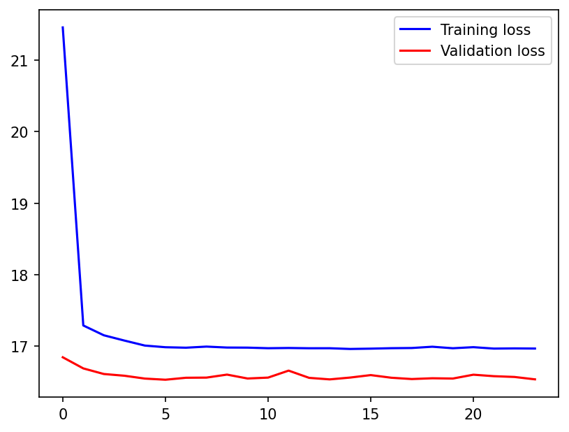
Visualizing the Results#
Comparing the training and validation loss curves
plt.figure(dpi=150)
plt.plot(train_loss, "b", label="Training loss")
plt.plot(val_loss, "r", label="Validation loss")
plt.legend();
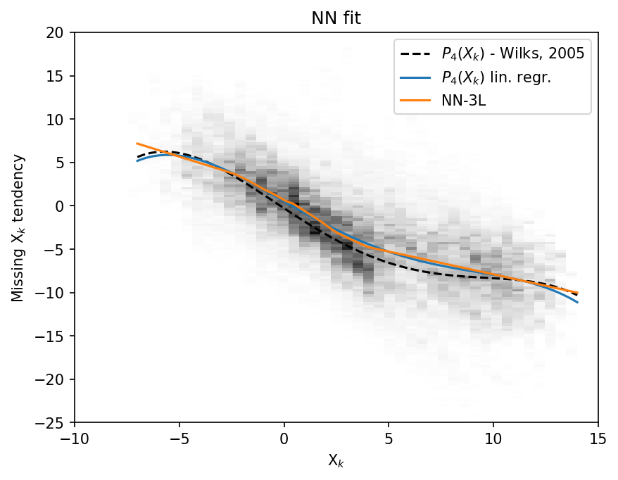
Since the NN has one input and one output, we can plot it as a function \(nn(X)\) (orange), and compare it to the polyfit (blue) and Wilks 2005 polynomial (black dashed).
plt.figure(dpi=150)
plt.hist2d(
    x_input.flatten(),
    X_tend.flatten(),
    bins=(np.linspace(-10, 15, 50), np.linspace(-25, 20, 150)),
    cmap=plt.cm.Greys,
)
plt.plot(x, -np.polyval(p18, x), "k--", label="$P_4(X_k)$ - Wilks, 2005")
plt.plot(x, np.polyval(p, x), label="$P_4(X_k)$ lin. regr.")
plt.plot(
    x,
    (nn_3l(torch.unsqueeze(torch.from_numpy(x.astype(np.float32)), 1))).data.numpy(),
    label="NN-3L",
)
plt.legend()
plt.xlabel("X$_k$")
plt.ylabel("Missing X$_k$ tendency")
plt.title("NN fit");